Spinal vertebrae localization and analysis on disproportionality in curvature using radiography—a comprehensive review

Abstract

In human anatomy, the central nervous system (CNS) acts as a significant processing hub. CNS is clinically divided into two major parts: the brain and the spinal cord. The spinal cord assists the overall communication network of the human anatomy through the brain. The mobility of body and the structure of the whole skeleton is also balanced with the help of the spinal bone, along with reflex control. According to the Global Burden of Disease 2010, worldwide, back pain issues are the leading cause of disability. The clinical specialists in the field estimate almost 80% of the population with experience of back issues. The segmentation of the vertebrae is considered a difficult procedure through imaging. The problem has been catered by different researchers using diverse hand-crafted features like Harris corner, template matching, active shape models, and Hough transform. Existing methods do not handle the illumination changes and shape-based variations. The low-contrast and unclear view of the vertebrae also makes it difficult to get good results. In recent times, convolutional nnural Network (CNN) has taken the research to the next level, producing high-accuracy results. Different architectures of CNN such as UNet, FCN, and ResNet have been used for segmentation and deformity analysis. The aim of this review article is to give a comprehensive overview of how different authors in different times have addressed these issues and proposed different mythologies for the localization and analysis of curvature deformity of the vertebrae in the spinal cord.

1 Introduction

1.1 Spinal cord and its properties

The central nervous system (CNS) is the most important processing unit in human anatomy. It manages and controls all the essential organs from head to toe naming eye blinking, breathing, heart pumping, and movement of motion including bending and twisting. CNS has two major organs; the supreme one is the brain, and the subsequent is the spinal cord. CNS works like human central processing unit (CPU) of a computer system as it monitors and transfers information from the brain to the rest of the body with the help of the spinal cord. The starting point of spine is the brain stem. The spinal cord is a delicate vertical tube-like pipe with a firm texture that contains a bunch of nerves and tissues. Nerve bundles are of two types: the information sensory known as sensory roots and the signal transferring known as motor roots [1]. The edge of the spinal cord is termed as cauda equine because of its similarity to the horsetail.

1.2 Spinal cord significance

The nervous system is a vital body phenomenon. Taking one of its major organs, the spinal cord, and describing its significance are a crucial task. The damage in the major hub of information transmission network can disturb the functionality of any other vital organ. The spine nerves along with sensory signals transmit information signals to other parts of the body. They are the main communication system of the human body, as it connects each organ and its response to the brain. The brain, being the processing unit, gets and supplies all the information with the help of the spinal cord. The spine helps in mobility of the body. Any minor glitch or deformity in the spine can lead to complete paralyses. Our body has the capability to respond abruptly in any unexpected case. In simple words, our reflexes are controlled with the support of the spinal cord [2].

1.3 Spinal structure and movement

Fundamental anatomy of the spinal cord, as shown in Fig. 1, begins from the brain with an estimated length of 40–50 cm and a width of 1.0–1.5 cm. This fragile tube ends at the hip bone. The ideal spine curves contain 31 nerves. These spinal nerves have white-grayish matter with five divisions: (1) 8 nerves of the neck cervical, (2) 12 nerves of the chest thoraces, (3) 5 nerves of the abdomen lumber, (4) 5 nerves of the pelvic sacral, and (5) 1 tailbone nerve coccygeal. The spinal cord has 3 layers of tissues: the innermost layer is pia, the middle layer is arachnoid, and the outermost layer is dura. The structure of the spinal cord contains a series of 33 small bones stacked upon each other known as the vertebral bone [4]. The soft mushy material between each vertebra is the disc that creates the shape and pattern of the whole spinal cord. It handles one of the crucial mechanisms which is the connectivity of the brain and spinal cord for the communication process of the body [4].

Fig. 1

The human spinal cord [3]

2 Spinal posture deformilies

The issues regarding the spinal cord is an extensive topic. However, the common symptoms that indicate spine problems include weakness, senses loss, sweating, swelling, numbness, bladder control, reflex action, paralysis, and back ache. Taking these symptoms into account, the clinical specialist can identify the affected. Causes behind these issues can be the infection, trauma injury, vascular blockage, bone fracture, and tumor [5].

The deformity of the spine is split into three categories. Figure 2 clearly depicts each category compared with normal spinal curve:

• 1. Scoliosis

  Fig. 2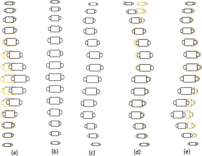

  

  Spine abnormalities. a Scoliosis. b Normal front view. c Normal side view. d Kyphosis. e Lordosis

• 2. Kyphosis

• 3. Lordosis

2.1 Scoliosis

One of the sideways curvature deformities of the spine that occurs commonly during the growth and erupts just before puberty is called scoliosis. Most of the time, cases of scoliosis are mild, but with the passage of time, spine scoliosis deformities get severe as a child grows. The severity of scoliosis can lead to disability [6]. Especially, extreme curvature disorders reduce the space within the chest, that causes breathing problems as it effects the functionality of the lungs and heart. Chronic back pain and uneven shoulders, hips, and waist are the common symptoms of this case. Wearing a brace is one of the solutions to stop the increase in scoliosis while another method to keep curve deformity from worsening is surgery. In a study [6], the authors have explained scoliosis causes and its effects. The fluid gathering and its proliferation in the central canal of the spinal cord result in chronic pain in the neck, along with a feeling of fatigue and loss of sensation. In [7], detail discussion on scoliosis curve defects is mentioned with two basic shape-based categories that are “S’ and “C’ curves. The authors split the disease on the basis of thoracic, lumbar, cervical and took 79 cases of idiopathic lumbar scoliosis, 26 thoracic lumbar, 134 thoracic, and 69 combined cases for study finding 3–4 curve patterns.

2.2 Kyphosis

Kyphosis is the over elaborated round-back from the cervical region. In simple words, it is a vertebrae wedge-shaped deformity from neck to shoulder. Kyphosis can occur at any age, even in infants, but it is mostly common in older women. There are three types of kyphosis: (1) postural is the most common, (2) Scheuermann is a severe category of hyper kyphosis, and (3) congenital is by birth and happens when the spinal cord fails to develop normally. Mild kyphosis causes a few issues such as stiffness, breathing and digestion problems, and back pain. The severe kyphosis can cause pain and be disfiguring, so it increases the chances of diseases like fracture, disgeneration, osteoporosis, and cancer. Due to kyphosis, the curvature change is more than 50 ^∘. In article [8], Sinaki et al. described the disease by explaining the changes in the Cobb angle from 50 to 65 ^∘, making it hyperkyphosis. The authors combined image analysis of patients, along with gait analysis to study the clinical deformity and perform a detailed statistical analysis as well. The study proved that patients of osteoporosis have more chances of having hyperkyphosis. Gait analysis showed that poor balance and stubby gait might cause any kind of serious fall.

2.3 Lordosis

If the lower lumber pelvic curve, which is above the buttocks, arches too far inwards, it is called Lordosis. Lordosis can cause excess pressure on the structure of the spine causing severe pain and discomfort, and it can also effect the subject’s movement. Treatment of lordosis depends upon the severity. In mild cases, one can improve their condition with physiotherapy and exercises. The excess in the arches of the curve is called swayback. It is common in children but often gets better with growth. This kind of lordosis is termed as benign juvenile lordosis. Spondylolisthesis can be one of the reasons behind lordosis. It can be by birth or may develop after certain athletic activities. Levine and Whittle in [9] explained the lordosis, stating that the immoderate inward deformation of the lower back curve is lordosis. The authors explored the slant of pelvic lumber curve, which can be due to excessive standing. Their study showed that three pelvic parameters are standing posture, maximal anterior, and posterior pelvic tilt. Increase in anterior tilt results in the rise of the depression in the spine. Thus, the study results depict that a person can significantly alter their pelvic angles because of lumbar lordosis.

3 Diagnosis techniques

Spinal curvature disorders and abnormality diagnosis in patients can be done through three different ways. The first one is physical examination which includes physical check-up, palpitation check-up, and observation of gait motion. “Adams Forward Bending Test” is also one of the famous techniques in physical diagnosis [10]. The second one is neurological evaluation which involves the severity assessment of symptoms and pain, muscular spasm, weakness of the bladder, and motor evaluations. The third one, which is the most popular and reliable method for diagnosis of spine deformity, is through radiological images. This diagnostic method gives clarity of the organ and helps to identify the severity level.

3.1 Radiological diagnosis

A number of imaging modalities are available for analysis and diagnosis of spine posture issues. The famous and cheapest among all is radiography images, which are shown in Fig. 3. With the evolution in technology for detail study analysis, a number of options are available such as X-ray, computed tomography (CT) scan, magnetic resonance imaging (MRI) scans, positron emission tomography (PET) scans, and single-photon emission computerized tomography (SPECT) scans which are the prominent ones for the evaluation of the spinal column. Some of these imaging modalities are expensive, and for some medical specialists, a prescription is compulsory as if possible, unnecessary radiations can be avoided [11].

Fig. 3

Spine X-ray, MRI,and CT scan

3.1.1 X-ray images

Wilhelm Conrad Roentgen in 1895 discovered an X-ray technique that is electromagnetic waves-based radiations that can capture and help to visualize the internal body structure [12]. The bombardment of radiation to the body and bone material calcium naturally absorbs these radiations generating bright whitish structure on image film. X-ray imaging of the spinal cord is a very popular and the cheapest method. The huge amount of research work is carried out on this imaging area [11]. X-ray image analysis helps to detect any spine issues related to the vertebrae column, fracture, and tumor.

3.1.2 CT scans

CT is another imaging modality for the analysis and diagnosis of spine disorders. It is basically a combination of advance X-ray images from multiple angles and orientations. These scans are processed with parameters of measurements and produce cross-sectional images of an organ from different sides. Nowadays, CT scans help to generate 3D models of the spinal cord. The clinical specialist can study the model with all scales and orientation shifts. The computed tomography technique was developed by a British, Godfrey Hounsfield of EMI Laboratories in early 1970s [11]. CT scan is considered a more reliable technique for detailed tissue and vascular analysis.

3.1.3 MRI scans

An acute high-quality and remarkably detailed method in radiological evaluation of the spinal cord can be achieved with an MRI scan. This non-invasive imaging technique produces images by creating a strong magnetic field and pulses of radio frequency [11]. MRI was discovered in 1946 by Felix Bloch and Edward Purcell. These scans require prescription by a clinical specialist. MRI scans are a bit expensive, and during scans, medical assistance for detail evaluation is compulsory.

4 Literature review

The literature review is discussed in a time series format. In the first section, the literature discussed is from 1960 to 1999, the second section of literature is from 2000 to 2015, and the last section is 2015 onwards. The paper selection was done on the basis of good number of citations and publication in prestigious journals and conferences.

4.1 Early literature

One of the earliest research papers for cobb angle calculation was by Flint [13] in 1963. The author carried out a study on 31 female college students of age 19–22. The purpose of the study was to determine the correlation between the flexors and extensors of the pelvic hip and to measure the significance of abnormality of the back muscle on lumber posture. Two images of the subject standing behind a mesh of a 2 × 2 screen in a relaxing position. With the help of previous studies, the plumb line for both images was dropped to measure the line of gravity. The radiologist helped in detecting the focal point of the trochanter. Placing 4 landmark points at the spine, over the sacral and lumber junction, over the upper surface, and one over the dorsal surface of the sacrum. Drawing the first line from the dorsal to the apex of curve which intersects the line upwards from sacrum pointers, the STL2 angle on the intersection was the reading. The second reading was taken from the angle taken from the intersection of the lines paralleled to the pointers on the inner-lumbar surface with the sacrum outer surface. This L angle was taken to measure lordotic curve. Larger value of the angle reading indicates a smaller curve and vice versa. PI2 angle of pelvic inclination was calculated by an angle formation between the pelvis horizontal plane and horizontal line from the anterior and the posterior superior iliac spine. For performance measure, the mean and standard deviation for each set and coefficients of correlation between the curve were calculated. STL2 values are not significantly correlated; L2 suggests flexibility of the hip does not impact on the lumber curve. The author stated three basic conclusions; the first is the external measurement for the lumbar provides an accurate measurement of lumbar convexity. The second is that, there is no significant relationship between lumbar lordosis with hip-trunk flexibility. Third is that pelvic inclination which has no impact on the position of the center of gravity.

In 1967, Loebl wrote a paper [14] for the measurement of normal spine posture using rheumatology images. The dataset used was of 176 spine images of age 15–84 years from Westminster Hospital and Queen Mary’s Hospital, Roehampton. The position of subjects for images were sitting, standing, and bent. Inclinometer was used with a 9-cm gap and scale set to degree. Keeping weight needle remain vertical indicated the angle of spine inclination. The spine downward pattern was marked in intervals from D1 to D12. Spine segments were split in four divisions excluding the neck: upper and lower dorsal with dorsa-lumbar junction and lumbar. Nine normal subject’s readings were taken 5 times; 14 ^∘ average variation was observed. The variation was due to manual inaccurate readings. For the dorsal spine below age 40 females have a curve 4–5 ^∘, straighter than men, but for age above 40, the bent of both genders is almost same. The lumbar curvature varied from 25 to 55 ^∘ ± 7^∘ in old age. The author emphasized on the importance of curve variations like deep lordosis is due to hip deformity. Thirty-eight rheumatoid arthritis patients measured have no difference from normal ranges, and 15 ankylosing spondylitis results were the same. Only one patient with scaro-iliac joint having a 12 ^∘ difference confirmed dorsal spine effected. Improvements were observed after exercise and phenylbutazone. The concluding remark of the author suggests that maximum subjects have accurate angle within 10% of normal ranges.

Mehta [12] discussed the disease scoliosis using radiographs. The convex side of the vertebrae was then rotated in a clockwise direction through an arc of 90 ^∘ with intervals of 15 ^∘. Producing a series of images with a remarkable variation in appearance. The change in the interval less than 15 ^∘ failed to produce a clear difference. Multiple landmarks on composite images were drawn to get a rotation difference. The transverse process is the difference between ranges of 15–30 and 45–60 ^∘, which was helpful, but the difference from 75 to 90 is almost the same. The study was carried out for scoliosis images as well determining the extent of curvature change. The image matching method was proposed for the estimation of disease. The methodology provides approximate results but gives a plus point to monitor rotation to 90 ^∘.

Levine and Leemet [15], in their paper put an idea of two stage approximations edge detection. To determine where the spine is located, vertical signature of the entire image is taken, and a smoothing method is applied to reduce noise. Later, for edge detection, horizontal scale first derivative was computed and least square polynomial fit was applied in the second stage. To restrict local search of edges mean predictive weighing function improved the process. The polynomial fit order was increased from third to fifth order in an iterative manner for better results. Lastly, the center line was calculated with the help of the median of both edges on a horizontal scale. Chwialkowski et al. [16] in their research article revealed the quantitative measuring strategy for lumbar disc evaluation. The proposed method utilized 12–15 sagittal images; edge enhanced rectangular block with spine size for region of interest (ROI) was specified later. A morphological model of the vertebral structure was designed as a vertebra candidate fitting block was localized. The center-most cluster part of each candidate fitted was considered as an estimated inter vertebral disc. Intensity profiling of each estimated area of disc space is carried out along with the bisection line. For normal belly shape, the intensity curve was cross-compared, and there was an excessive difference that eliminates the abnormal disc. The average gray level 5 × 5 neighboring estimates the width of disc. Tagged findings will verify inconsistent trends in sequences to confirm abnormal discs.

In [17], Smith et al. described usage of active shape models (ASM) to locate the vertebrae in DXA images. These low-spatial resolution images contain noise, providing a challenge for object localization. All vertebrae in the image were marked manually with six points for each from thoracic T7–T12 and lumbar L1–L4. Similarly, point distribution models (PDM) were applied in addition with PCA for simplification of the covariance matrix. Basically, ASM uses both shape-based and gray-level appearances for the detection of objects in image. The results were characterized as a Gaussian distribution with the help of the EM algorithm. Rejected cases were eliminated if their error lays above μ + 3 σ of the successful cases.

The domain of image processing emerged in the late 1960s. That early era of image processing mostly focused upon enhancement and restoration of images. For the medical domain, image acquisition and dataset collection were the major issues for the researchers. This early era of research indicates problems such as low-quality images and limited availability of imaging modalities. The immaturity in the domain was the key factor, and a limited number of available techniques for segmentation and classification are also one of the drawbacks. Roentgenographic [18] and X-ray images were mainly used for differential diagnosis. Morphological processing was popular for extraction of components from images. One of the secondary issues in that era was the limitations of the hardware, such as storage spaces, memory issues, and smaller cycles per second of the processor, leading to low capacity as a whole for complex processings.

4.2 Mid-era literature

Brejl and Sonka in their research article [19] proposed the new method using model-based image segmentation. The authors utilized 2D MRI with different dimension of the thorax brain and spine. The training dataset has manual boundary tracing in combination with landmark identification. For contour alignment of training data, the mean and variation shape are set in R-table. Another border appearance model was designed for training dataset. Shape-variant Hough transform and edge-based object segmentation were used for segmentation.

In [20], a report is generated about the development of a segmentation technique using 50 NHANES II X-ray images, for positioning and orientation of the cervical vertebrae. Every image landmark is identified on the basis of morphometric points identified with the assistance of an expert radiologist. The technique is claimed to be noise, rotational, and scale invariant. The generalized Hough transform (GHT) is customized to provide the shape information using its mean and corresponding templates. The built-in accumulator structure helps to deal with noise. The given techniques provide orientation and location along with contour of cervical vertebrae. The average 72.06 out of 80 LMP falls in the boundary box, and the orientation error was average 4.16 ^∘.

Gamio et al. [21] proposed a novel research approach for vertebral segmentation from MRI scans. The dataset consists of 6 subjects. Initially, coil correction is applied. It is followed by interpolation with mean values of adjacent slices that generated a 3D stack. Normalization followed by the cropping of the region of interest facilitates to reduce size and computations. Anisotropic diffusion algorithm is used to reduce brightness and for preservation of edges. Normalized intensity based on 3D local histogram provides brightness features, and histogram of texton gives position and intensity features for segmentation. For the localization of the spine bone, normalized cut technique was utilized after that Nystrom approximation method was implemented for vertebral body segmentation. This helps in the determination of results on the bases of difference in nk the number of bins with the rp and rz size of the local volume for histograms.

Peng et al. [22] discussed an algorithm for vertebra segmentation using MRI scans. The proposed algorithm has two stages; the first one is inter-vertebral disk localization, and the second one is vertebra segmentation. In the first stage, the localization is done with the help of a model-based search method which gives clues regarding inter-vertebral disc spaces that are adjacent to each vertebra. The intensity profiling on polynomial function is used to refine and verify the candidate disc spaces. The center point of the disc with extended profiling in the horizontal direction will provide shape approximation. Later, a canny algorithm is used for the boundary extraction of the vertebra. Recalculation of disc space with the help of boundary values and repeat polynomial profiling will identify inter-vertebral disk distances. Seven subjects MRI scans of 412 × 1012 resolution. Successful boundary extraction of 22 vertebrae for 5 datasets is approximately average 94%.

Lin in his research article [23] formulated a 3D spine model with the help of coronal and sagittal planes. Seventeen uniformed segments and 18 nodes with 3D Bezier curves fitting were superimpose over X-ray scans. Plot from top to bottom, an axial view of the space curve was produced. The features selected by the author were curvature and torsion. To evaluate spinal deformity, King’s classification was applied along with multilayer feed-forward, back-propagation (MLFF/BP) artificial neural network (ANN). Dataset of 37 X-rays with a subset of 25 training and 12 testing images, splitting subgroups of training 5 kings [24]. Results for two hidden layers identification rate rn = 0.68 at 300 iterations and then elevated to rn = 0.84 at 900–1200 iterations and for one hidden layer identification rate rn = 0.72 at 300 and 1800 iterations to rn = 0.76 at 1200 iterations.

Xiaoqian et al. in [25] utilized 801 cervical and 972 lumbar X-ray images from NHANES II. The researchers studied a nine-point landmark model which the clinical experts used to explain vertebra shapes. Xu et al. established an automatic system which detects those nine-point model on the basis of their semantic heuristics. Corner information provided by this automatic system has been the initial input for proposed partial shape matching (PSM) using dynamic programming. To reduce the number of data points to 20 vertices, the technique of curve evolution is applied. By eliminating the negative angle, which points in the clockwise direction, positive bend angle might be the corner of a vertebra, creating a line segment between two points on the contour. Using DP, each point set triangle data is saved for every classification matching is carried out from the dataset. A total of 801 cervical and 972 lumbar segmented shape dataset was formed from a total of 400 X-ray images.

Benjelloun and Mahmoudi in [26] performed a comprehensive analysis for the extraction of anterior left faces of the vertebra contour. They focused on extracting angular variation in combination with the spine column and by computation of angles for global curvature. They rely upon Harries’ interest point detector for key points. For mobility analysis using supervised one click corner of the vertebra, the left boundary is extracted. Encircling the point clicked, research zone direction tangent is determined. The distance between two corners inside the circle is measured and is supported by pre-processing. Contrast enhancement gives better results in corner recognition. A dataset was used of 100 images from the National Library of Medicine providing stability, speed, and satisfactory results.

Tobias et al. in their research article [27] described a framework for vertebrae detection and segmentation using CT images. The methodology started with curve extraction using sophisticated generalized Hough containing parameters of multiple shapes and a number of objects. The vertebral coordinate system describes the location and coordinates of vertebra in combination with a seed point progressive adaptation method. For the identification of vertebra, average intensity information inside each vertebra bounding box was utilized, and for segmentation of every single vertebra, adapting triangulated shape models was applied.

In [28], Ribeiro et al. used 40 cases from which 19 are confirmed fractured bones and 22 normal spinal images. Gabor filter bank with 180 filters was applied on these gray-scaled images at angles θ = - π/2. Resultant data provides fine orientation details due to high response over edges and corners. The response then later weightage calculated by addition of sine and cosine of twice of significant angle. In the center of the vertebra, points were marked using a mouse for distance calculation and region splitting. Using the neural network, the logistic sigmoid function for more detailed analysis, along with that morphological opening and closing, is carried out for holes, noise, and region filling. The accuracy of the proposed system is quoted to be in the range of 91–92%.

Anitha and Prabhu in [29] proposed a methodology for automatic quantification of spinal curvature using 250 radiographs. They split the radiographs in group category on the basis of degree of Cobb angle. They initially enhanced the input image, then Snake-I methodology calculates the initial boundary to make it less sensitive to noise gradient vector field; Snake has provided better results. The boundary that is extracted has been enhanced and retained using some morphological operations using a structuring element. Hough transformation has calculated the slope of the horizontal lines of boundary. This has given exact information about vertebrae eliminating inter/intra-observer error.

In [30], Larhmam et al. claimed 89% accuracy in their approach where they studied out of 200 images of 40 healthy cases and validated the result. They used Hough transformation based on a modified template matching methodology. This method is translation-, rotation-, and scale-invariant. For segmentation, the first step was model construction on geometry of average of 25 vertebras. In the second step, canny was applied and Gaussian smoothing was used in combination with Sobel operator and non-maxima suppression. Hough transform was the third step of the segmentation process to reduce false-positive edges. Vertebra potential center identification is carried out through contrast limited adaptive histogram equalization (CLAHE) in line with Canny and Sobel for edge detection. Finally, on Hough R-Table, linear regression selects the highest voted point.

Sardjono et al. in [31] highlighted the Cobb angle determination using 36 X-ray images. The authors underlined Jalba et al. CPM technique from 2004, for the vertebra edge detection. Charged particle method provides segmentation based on charged particles attracted to the contour of the object whose gradient magnitude had helped to locate the boundary on the object. To identify the S curve, three parts of the spine in the vertical direction had determined two angles of Cobb, while for C curve, two parts of the spine had identified a single Cobb angle. Piecewise linear curve fitting method with a slope of curve in line with splines, steps, and polynomial function had determined Cobb angle. On 36 X-ray images, R2 is measured with different segments and steps providing satisfactory results.

Rasoulian et al. in [32] suggested a novel shape pose segmentation technique. The dataset used for processing consist of 32 CT images acquired from Kingston General Hospital and Vancouver General Hospital. Using group-wise Gaussian mixture model (GMM) based on registration technique boundary was established. To obtain statistical shape, the principal component analysis (PCA) helped in parameter selection. Expectation maximization registration algorithm of segmentation was used. Sorting of eigenvalues and weights to PGs improved registration speed. To smoothen CT scans, the multivariant Gaussian kernel was utilized in combination with a canny edge detector to produce boundary. Results calculation: The matric mean of point-to-surface distance error was computed to be 1.38 ± 0.56.

The first decade of the new millennium was significantly good for DIP as the domain was gaining both popularity and maturity. The increase in demand of medical imaging, improved quality of images, and multiple accusations and enhancement methods opened the doors for reliable diagnosis. Nevertheless, the noise in medical images, low contrast, and brightness issues were the main problems highlighted by researchers. Thus, better ways of preprocessing were introduced. Many new filters and noise removal techniques were applied to improve results. The evolution in the hardware industry also facilitated in the processing and storage solutions. Novel segmentation and classification techniques were introduced and applied on medical imaging which enhanced the results by leaps and bounds.

4.3 Recent literature

In a study [33], Korez et al. developed an automated supervised segmentation method for vertebral bodies with the help of 3D convolutional neural network (CNN). The dataset consisted of MRI scans of 23 subjects, 3D mesh of mean shape model of vertebral body formation. Later on, CNN supported to provide generalized probability map of VB. Figure 4 shows their entire model. The actual novelty of the proposed technique is 3D spatial VB probability maps. For the evaluation of the proposed methodology, the dice similarity coefficient was calculated 93.4 ± 1.7%.

Fig. 4

Spatial vertebral body and probability maps [33]

To reduce the misdiagnosis from CAD systems, Arif et al. in their research article [34] proposed a fully automated cervical segmentation framework using a deep, full CNN. With the help of probabilistic spatial regression, localization of the vertebrae center is done. For segmentation, datasets from Royal Devon and Exeter Hospital containing 124 X-ray images in training and 172 in test data were utilized. Without any manual input, a shape-aware deep network was formulated. Evaluation metrics achieved dice similarity coefficient of 0.84 and a shape error of 1.69 mm.

In the paper [35], Shi et al. developed two leveled methodology for vertebral localization and segmentation with the help of the intensity pattern in combination with CNN for GPU accelerations. In the initial step, spinal region extraction is carried out using 2D U-Net variants. Later, for each vertebrae, centroid localization is done by applying M-methodology which resulted in producing a 3D ROI. Later, with inception 3D U-net was utilized, training on 61 annotated CT images. The correct identification of 92% and error rate of 0.74 mm with 0.8mm of dice coefficient was achieved. In [36] paper, Lu et al. described a fully automated deep-learning approach for lumbar spinal stenosis grading. The research provides three major contributions: first, NLP scheme to extract level-wise ground truth labeling from radiological reports of multiple types and grading of spinal stenosis; second, disc-level vertebral segmentation and localization using an U-Net framework in combination with a spine-curve fitting; third, contribution was usage of multi-input, multitask, and multi-class CNN to execute central canal and stenosis grading. Massachusetts General Hospital (MGH), Department of Radiology, gave lumber MRI dataset of 22,796 disc levels extracted from 4075 patients. The proposed algorithm gives an accuracy of 94% for both the spine canal and foraminal stenosis.

In [37] paper, automatic landmark localization using the WHDV method that includes U-Net architecture of CNNs was used. For the training of CNN, a modified version is used for estimation Gaussian response known as “heatmap only” around each target, using predictions to vote for the point position. For evaluation, dataset of 1696 radiographical images of child hips age 2–11, including both cases of normal and diseased was used. Experimental result accuracy shows significant improvements in comparison with the RFRV-CLM method, having a median error of 6.92% and 5.85%, respectively.

Kim et al. in [38] proposed a novel semi-automatic segmentation algorithm for the vertebrae in lumber MRI. After extraction of ROI for each vertebra, specify the parameters with the help of a correlation map. ROIs are tuned with Hough transform and canny edge filtering. Later, segmentation is carried out via graph-based and line-based algorithms. Algorithm testing on lumbar sagittal MRI dice similarity coefficient reached to 90%, in comparability with manual.

Rehman et al. [39] discussed the CAD system for accurate vertebrae segmentation with the help of region-based deep learning. Modified form of U-Net with level ant and combination of shape prediction are applied. They are termed as FU-Net framework. Training network was applied on 500 epochs with early convergence which achieved 0.9 momentum learning rate and 0.2 dropout among two adjust layers. For all experiments, 2D sagittal slices are applied and to improve learning performance data augmentation is compulsory. The proposed methodology produced 96% dice score and 0.1 ± 0.05 absolute surface distance on two different datasets of CSI 2016 and CSI 2014.

In [40], the issue of vertebral segmentation has been discussed along with detection of vertebral abnormalities. The research emphasized on paradigm of deep learning on medical images. Chuang et al. suggested an iterative segmentation model 3D U-Net and DeconvNet that segments all categories of vertebrae, which includes the cervical, thoracic, and lumbar vertebrae. The authors have used xVertSeg dataset. Cross-entropy is used as loss function for the multi-label classification. The authors claimed better performance from previous methodology of Lessmann et al. and is memory efficient as it used 17% less memory.

Lessmann et al. in there article [41] addressed the vertebrae segmentation and identification of abnormalities. They proposed an iterative approach by using fully CNN to segment and label vertebrae. The following are the four major components of the authors’ approach: (1) segment voxels from a 3D patch, (2) instance memory, (3) identification sub-network, and (4) completeness classification sub-network. Dataset computational spine imaging (CSI) of 2014 and thoracolumbar spine CT is utilized. Average dice score of segmentation 94.9 ± 2.1% and 93% correct anatomical identification. Figure 5 presents some of the segmentation results.

Fig. 5

Segmentation results of [41]

Aubert et al. in their paper [42] proposed automated 3D spine reconstruction technique. A total of 400 images training dataset with a mean Cobb angle o 43 ^∘ having idiopathic scoliosis was taken from Saint-Justine University Hospital. The statistical spine shape modeling that depicts global view of spine curve along with local shape of vertebra. It has geometrical exhibition using simplified parametric model (SPM) of the vertebra. Spinal cord automatic landmark detection is carried out using CNN patch-based regression. Strategy named coarse-to-fine was formulated for automatic 3D reconstruction. The landmark mean (SD) location error from 3D Euclidean distances were 1.6 (1.3) mm from the vertebral body center, 1.8 (1.3) mm from the endplate centers, and 2.3 (1.4) mm from the pedicle centers. In the latest era, last 4 years of research was discussed indicating great work and progress in medical imaging. The research in these years indicates the usage of different CNN architectures. The popular CNN method is commonly used for segmentation. CSI datasets are in demand for spinal research. Notably, CNN dominates but require a lot of images for good training and testing. Medical data is hard to collect and that data also require medical assistance for annotation and labeling. With great progress in the results, no imaging technique is free of noise. Therefore, issues like illumination, artifacts, and low contrast effecting segmentation require attention to improve results.

Pasha et al. [43] conducted a research study from X-rays of 103 adolescent idiopathic scoliosis patients. 3D spine model was used to measure clinical parameters such as thoracic Cobb, lumbar Cobb, sacral slope, pelvic tilt, thoracic kyphosis, and lumbar lordosis, by connecting the T1–L5 vertebral centroids to formulate 3D curve. To normalize spine heights, isotropic scaling was carried out. A total of 17 Z level were calculated with the help of T1–L5 coordinates which produced a normal spine cohort. The agglomerative hierarchical clustering was used to merge similar spines in one cluster. The difference in clusters identifies the maximum dissimilarity with normal spine. Almost 3 anatomical views of spine were determined in each cluster. The results indicated 5 different 3D curves in right thoracic; maximum dissimilarity was in patients of hypo-thoracolumbar kyphotic (44%) and flat sagittal profile (56%). Both sagittal and frontal imbalances were found.

In 2019, Chen et al. [44] proposed to use a 3D Full CNN in combination with hidden Markov model (HMM) for the identification localization of the vertebrae. The authors utilized 242 CT scans for training along with 60 scans for evaluations from public dataset of MICAAI challenge. Initially, FCN was used for training and detection of vertebra centroids. Second, FCN network was formulated for both local and global information from scans, this classification network handle indexing of vertebrae. The authors proposed post-processing strategy to increase the robustness and to achieve high-level optimization HMM. Experimental results on test data produced a mean identification rate of 87.97% and a mean error distance of 2.56 mm. In [45] paper, Pastor et al. conducted a study on 232 CT scans with different arbitrary field views in a period of 12 moths. The dataset was split into two groups: 186 scans for training and 46 scans for testing. In the first stage, a manual centroid annotation is done. In the later stage, learning-based decision forest method was implemented. Detection procedure was based on random regression forest (RRF) for localization and identification of the vertebrae. Voxel-wise operations are applied for the improvement in results. Image binarization and dilation followed by logical NOT were performed achieving the identification rate of 79.6%.

Vergari et al. in their research [46] proposed a classification technique for the automatic detection for scoliosis. The dataset originally consisted of 796 radiographs and was augmented up to 2096 images. Later, it was divided into 1892 training images and 204 validation images. The classification method was inspired from the architecture of LeNet-5. Three convolutional layers followed by batch normalization and max pooling layers in combination with dropout layer at the terminal. The results are further processed through discriminant analysis. This discriminant analysis refined and improved accuracy level of correct classification rate up to 96.5%.

In 2020, Alharbi et al. [47] evaluated their approach for automatic scoliosis angle calculation with 243 images dataset supported from King Saud University, Riyadh, Saudi Arabia. The performance evaluated reached to 90% accurate detection. The authors used the CLAHE method in preprocessing to enhance the X-ray quality. The ResNet CNN framework was utilized for the detection of the vertebrae. Transfer learning supports the algorithm results. Cobb angle measurements were calculated after corner of each boundary box help to calculate the center point. Measuring line angles between each center of the vertebrae to find angle the y-axis is measured by addition of 90 ^∘ and subtracting it from 180 if the resultant angle gets greater than 90 ^∘. The difference of minimum and maximum line angle produce a Cobb angle. The algorithm used novel approach to calculate the Cobb angle, with a small difference of 5–10 ^∘ from a clinical way.

5 Discussion

In this section, we present the review analysis of all the literature studied. The comprehensive literature review was split into time series format. In the first stage, 20 years of research work in this domain was studied thoroughly indicating several basic challenges. Image processing was not established at that time, with very limited techniques such as basic morphological operations and manual inputs; it was very difficult to produce good results. Secondly, the lack of resources like dataset and image accusation and its quality were the drawbacks in this area of study. Furthermore, this tenure produced great work like M. H. Mehta in 1973 proposed a traverse process and image matching in order to detect change in the curve. Intensity profiling for inter-vertebral disc recognition was proposed by Chwialkowski et al. in 1989 which turned out to be a renowned method of that time. Smyth et al. in 1997 proposed another approach which was manual land marking and contouring followed by usage of active shape model method on X-ray images. This proved to be another successful method of the era.

In the second tenure, related research work was better as compared with early era as shown in Table 1. The work in medical imaging was gaining popularity. Therefore, it increased the amount of research work carried out in this domain. The automated clinical assistance perspective attained acceptance, and the image processing domain was growing day by day. Artificial intelligence became the apple of the eye. Huge funding and projects started and that, in turn, started a new wave of algorithms and techniques in applied research. In Table 2, different research articles are mentioned, and we juiced it up with some highlighted points in those articles. For example, techniques like Hough transform, shape matching, curve fitting, EM, Gabor, and canny filters were star characters. They played a key role in almost every research article and gave reliable and improved results. The third phase of our comprehensive research consists of the last 5 years. The recent era opened a new chapter of neural networks. The research in these years revolves around different architectures of CNN such as FCN, UNet, FU-Net DeconvNet, and random forest regression voting framework. These CNN architectures produced good results, and the authors have used mean dice similarity coefficient as an evaluation metric for results as shown in Table 3. CSI 2014 and 2016 are the most popular datasets, and the illumination changes in images have yet to be catered for, and still there is room for improvement in results.

Table 1 Summary of early era literature

Table 2 Summary of mid-era literature

Table 3 Summary of recent literature

In this article, we have discussed in detail the evolutionary model of medical imaging in the specific domain of spinal deformity. One of the most important aspects is noise in medical imaging; one should not forget that radiographic images mainly have a wide range of noise issues that commonly affect the automatic detection and recognition of diseases. Different researchers address these issues and proposed multiple novel image enhancement techniques. Hsieh in 1998 [48] discussed the degrading in quality specifically about reduction in streak artifact due to photon noise in a radiographic image. The author proposed a random space-based adaptive filtering approach. Initially, the filter is applied on those color channels which exhibit photon starvation, as soon as the high signals are detected, the filter is stopped as it effects the resolution of the image. Secondly, smoothing is applied inversely proportional to photon signals. After these two steps, a resultant image appears as imbalance. To restore its balance, streak artifact reduction is used. To improve image appearance, adaptive trimmed mean filter for the reconstruction was applied. Nowak and Baraniuk in 1999 claimed that a major source of error in photon images is Poisson noise [49]. They performed an experiment to formulate wavelet-domain filtering. The filter adapts both signal and noise. 2D wavelet transform of photon image is computed with the help of filter H wavelet-domain filter version if image is established. Later, wavelet shrinkage is applied, followed by a press-optimal wavelet-domain filter. The authors conducted bone image study. High-intensity regions indicated that uptake of blood damages the bone. In 2003, researchers presented noise suppression technique for MRI scans using wavelet-based multi-scale products thresholding MPTH scheme [50]. Bao and Zhang in their study used canny edge detector like dyadic wavelet transform, which produced quick decay in noise and improved features evolving high magnitude across wavelet scales. To make most from wavelet inter-scale dependencies, the product of adjacent wavelet sub-bands is done to enhance edges while reducing noise. After that, adaptive thresholding was imposed on results which helped in identifying important features. In 2011, Gervaise et al. [51] evaluated the impact of adaptive iterative dose reduction (AIDR) and filtered back projection (FBP) for reconstruction of CT images. Different types of noise were studied such as CNR contrast to noise ratio, SNR signal to noise ratio, image noise, and spatial resolution. Fifteen CT lumbar spine scans were used; AIDR was tested on these images and compared with FBP for analysis of noise using evaluation metric Wilcoxon signed-rank test. The results showed up to 40% mean noise reduction. It also reduces the dose 52% of lumbar spine CT images.

6 Future work

The significance of the spinal cord and its deformity issues are already discussed above. Due to the global pandemic, as we are facing lockdown, majority of the work is being done from home. Sitting in bad postures for hours, while working from home, is damaging the spine curve. The spine deformity diagnoses at early stage through a reliable CAD system is required, so that we can avoid long-lasting damage in the spine. Deep learning algorithms in medical imaging can provide reliable results and provide detailed information regarding such issues. A good work in this area would be to develop an automated computer-aided diagnostic system for the segmentation of the vertebrae bone that is also able to provide deformity analysis on all the major categories, with respect to the difference in angle from normal spine curve. The improvement in segmentation results can provide better information regarding deformity. The noise and illumination problems in images also require a great deal of improvement. In addition to that, public availability of large datasets for the training and validation of convolutions neural networks needs attention. The CAD system can be an asset for the neurology departments of the medical institutes by assisting the clinical specialist to analyze the severity level of posture issues. This will be widely acceptable to the users as their problem will be addressed through a general test. It will also help them to follow the precautions to stop the increase in damage. The CAD system can also address other spinal issues such as fractures and tumors. This area of research is applied, and in third world countries like Pakistan, where there is a scarcity of medical resources, we require such research area to be promoted as these countries have a very low doctor to patient ratio.

7 Conclusion

This comprehensive literature paper presented an overview of the methodologies proposed for automated analysis of spinal deformities which is evaluated through vertebrae segmentation. Localization and segmentation of vertebrae have been the key research areas with the objective to distinguish between normal and abnormal curve of spine. This area of medical science has witnessed more then five decades of research, and this research article is an effort to give a thorough overview of work in all those years in combination with current state-of-the-art approaches on this subject. The segmentation of the vertebrae is a challenging task due to low-contrast and noisy images and problems like illumination changes and shape-based variations. The most popular clinical Cobb angle manual calculation was prime technique for measuring spine curve and to analyze its deformity. The deformity check requires neat vertebrae segmentation. The segmentation has been done by different researchers using different hand-crafted techniques like canny edge, Harris corner, template matching, ASM, and Hough transform. The variations in imaging modalities are also discussed and compared with techniques. Keeping current evolution of deep learning and CNN models, the most recent articles are solving this problem using deep learning models. These models can further be investigated more in detail by decoding the convolutional layers to specifically highlight the feature maps. This still needs to be explored in this area as mapping of features towards decision-making would contribute a lot in correlating automated diagnosis with clinical findings.

References

F. M. Maynard, M. B. Bracken, G. Creasey, J. F. Ditunno Jr, W. H. Donovan, T. B. Ducker, S. L. Garber, R. J. Marino, S. L. Stover, C. H. Tator, et al, International standards for neurological and functional classification of spinal cord injury. Spinal cord. 35(5), 266–274 (1997).
anonymous, Spinal cord injury: hope through research. https://www.ninds.nih.gov/Disorders/Patient-Caregiver-Education/Hope-Through-Research/spinal-cord-injury-Hope-Through-Research. Accessed 01 Aug 2019.
S. Ryan, Central nervous system stimulants and depressants. https://www.sralab.org/lifecenter/resources/spinal-cord-injury-what-it-and-what-does-it-affect. Accessed 01 Oct 2018.
R. S. Snell, Clinical anatomy by regions (Lippincott Williams & Wilkins, 2011). https://books.google.com.pk/books?hl=en&lr=&id=vb4AcUL4CE0C&oi=fnd&pg= PP2&dq=Clinical+anatomy+by+regions&ots=fMA9k57bJw&sig= pnJdMja1bbd0rS7lUz2lO3FFDzU&redir_esc=y#v=onepage&q=Clinical%20anatomy%20by%20regions&f=false.
M. Rubin, J. E. Safdieh, Netter’s concise neuroanatomy updated edition e-book (Saunders, Elsevier, 2016).
E. B. Sehlesinger, J. L. Antunes, J. W. Michelsen, K. M. Louis, Hydromyelia: clinical presentation and comparison of modalities of treatment. Neurosurgery. 9(4), 356–365 (1981).
J. I. P. James, Idiopathic scoliosis: the prognosis, diagnosis, and operative indications related to curve patterns and the age at onset. J. Bone Joint Surg. Br. Vol.36(1), 36–49 (1954).
M. Sinaki, R. H. Brey, C. A. Hughes, D. R. Larson, K. R. Kaufman, Balance disorder and increased risk of falls in osteoporosis and kyphosis: significance of kyphotic posture and muscle strength. Osteoporos. Int.16(8), 1004–1010 (2005).
D. Levine, M. W. Whittle, The effects of pelvic movement on lumbar lordosis in the standing position. J. Orthop. Sports Phys. Ther.24(3), 130–135 (1996).
anonymous, Adam’s forward bend test. https://tinyurl.com/y25644a9. Accessed 01 Dec 2019.
M. R. Nouh, Imaging of the spine: where do we stand?. World J. Radiol.11(4), 55 (2019).
M. Mehta, Radiographic estimation of vertebral rotation in scoliosis. J. Bone Joint Surg. Br. Vol.55(3), 513–520 (1973).
M. M. Flint, Lumbar posture: a study of roentgenographic measurement and the influence of flexibility and strength. Res. Q. Am. Assoc. Health Phys. Educ. Recreat.34(1), 15–20 (1963).
W. Loebl, Measurement of spinal posture and range of spinal movement. Rheumatology. 9(3), 103–110 (1967).
M. D. Levine, J. Leemet, Computer recognition of the human spinal outline using radiographic image processing. Pattern Recog.7(4), 177–185 (1975).
M. P. Chwialkowski, P. E. Shile, R. M. Peshock, D. Pfeifer, R. W. Parkey, in Images of the twenty-first century. Proceedings of the Annual International Engineering in Medicine and Biology Society. Automated detection and evaluation of lumbar discs in mr images (IEEE, 1989), pp. 571–572.
P. P. Smyth, C. J. Taylor, J. E. Adams, Automatic measurement of vertebral shape using active shape models. Image Vis. Comput.15(8), 575–581 (1997).
anonymous, Medical dictionary. https://tinyurl.com/y5qrkvsr. Accessed 10 Jan 2020.
M. Brejl, M. Sonka, Object localization and border detection criteria design in edge-based image segmentation, automated learning from examples. IEEE Trans. Med. Imaging. 19(10), 973–985 (2000).
A. Tezmol, H. Sari-Sarraf, S. Mitra, R. Long, A. Gururajan, in Proceedings Fifth IEEE Southwest Symposium on Image Analysis and Interpretation. Customized hough transform for robust segmentation of cervical vertebrae from X-ray images (IEEE, 2002), pp. 224–228.
J. Carballido-Gamio, S. J. Belongie, S. Majumdar, Normalized cuts in 3-D for spinal mri segmentation. IEEE Trans. Med. Imaging. 23(1), 36–44 (2004).
Z. Peng, J. Zhong, W. Wee, J. -h. Lee, in 2005 IEEE Engineering in Medicine and Biology 27th Annual Conference. Automated vertebra detection and segmentation from the whole spine MR images (IEEE, 2006), pp. 2527–2530.
H. Lin, Identification of spinal deformity classification with total curvature analysis and artificial neural network. IEEE Trans. Biomed. Eng.55(1), 376–382 (2007).
D. Ovadia, Classification of adolescent idiopathic scoliosis (AIS). J. Child. Orthop.7(1), 25–28 (2013).
X. Xu, D. -J. Lee, S. Antani, L. R. Long, A spine X-ray image retrieval system using partial shape matching. IEEE Trans. Inf. Technol. Biomed.12(1), 100–108 (2008).
M. Benjelloun, S. Mahmoudi, Spine localization in X-ray images using interest point detection. J. Digit. Imaging. 22(3), 309–318 (2009).
T. Klinder, J. Ostermann, M. Ehm, A. Franz, R. Kneser, C. Lorenz, Automated model-based vertebra detection, identification, and segmentation in CT images. Med. Image Anal.13(3), 471–482 (2009).
E. A. Ribeiro, M. H. Nogueira-Barbosa, R. M. Rangayyan, P. M. Azevedo-Marques, in 2010 Annual International Conference of the IEEE Engineering in Medicine and Biology. Detection of vertebral plateaus in lateral lumbar spinal X-ray images with gabor filters (IEEE, 2010), pp. 4052–4055.
H. Anitha, G. Prabhu, Automatic quantification of spinal curvature in scoliotic radiograph using image processing. J. Med. Syst.36(3), 1943–1951 (2012).
M. A. Larhmam, S. Mahmoudi, M. Benjelloun, in 2012 3rd International Conference on Image Processing Theory, Tools and Applications (IPTA). Semi-automatic detection of cervical vertebrae in X-ray images using generalized Hough transform (IEEE, 2012), pp. 396–401.
T. A. Sardjono, M. H. Wilkinson, A. G. Veldhuizen, P. M. van Ooijen, K. E. Purnama, G. J. Verkerke, Automatic Cobb angle determination from radiographic images. Spine. 38(20), 1256–1262 (2013).
A. Rasoulian, R. Rohling, P. Abolmaesumi, Lumbar spine segmentation using a statistical multi-vertebrae anatomical shape+ pose model. IEEE Trans. Med. Imaging. 32(10), 1890–1900 (2013).
R. Korez, B. Likar, F. Pernuš, T. Vrtovec, in International Conference on Medical Image Computing and Computer-assisted Intervention. Model-based segmentation of vertebral bodies from mr images with 3D cnns (SpringerCham, 2016), pp. 433–441.
S. M. R. Al Arif, K. Knapp, G. Slabaugh, Fully automatic cervical vertebrae segmentation framework for X-ray images. Comput. Methods Prog. Biomed.157:, 95–111 (2018).
D. Shi, Y. Pan, C. Liu, Y. Wang, D. Cui, Y. Lu, in Proceedings of the 2nd International Symposium on Image Computing and Digital Medicine. Automatic localization and segmentation of vertebral bodies in 3d ct volumes with deep learning (ACM, 2018), pp. 42–46.
J. -T. Lu, S. Pedemonte, B. Bizzo, S. Doyle, K. P. Andriole, M. H. Michalski, R. G. Gonzalez, S. R. Pomerantz, Deepspine: automated lumbar vertebral segmentation, disc-level designation, and spinal stenosis grading using deep learning. arXiv preprint arXiv:1807.10215 (2018).
A. K. Davison, C. Lindner, D. C. Perry, W. Luo, T. F. Cootes, et al, in International Workshop on Computational Methods and Clinical Applications in Musculoskeletal Imaging. Landmark localisation in radiographs using weighted heatmap displacement voting (SpringerCham, 2018), pp. 73–85.
S. Kim, W. C. Bae, K. Masuda, C. B. Chung, D. Hwang, Semi-automatic segmentation of vertebral bodies in MR images of human lumbar spines. Appl. Sci.8(9), 1586 (2018).
F. Rehman, S. I. A. Shah, M. N. Riaz, S. O. Gilani, R. Faiza, A region-based deep level set formulation for vertebral bone segmentation of osteoporotic fractures. J. Digit. Imaging. 33(1), 191–203 (2020).
C. -H. Chuang, C. -Y. Lin, Y. -Y. Tsai, Z. -Y. Lian, H. -X. Xie, C. -C. Hsu, C. -L. Huang, Efficient triple output network for vertebral segmentation and identification. IEEE Access. 7:, 117978–117985 (2019).
N. Lessmann, B. van Ginneken, P. A. de Jong, I. Išgum, Iterative fully convolutional neural networks for automatic vertebra segmentation and identification. Med. Image Anal.53:, 142–155 (2019).
B. Aubert, C. Vazquez, T. Cresson, S. Parent, J. A. de Guise, Toward automated 3D spine reconstruction from biplanar radiographs using CNN for statistical spine model fitting. IEEE Trans. Med. Imaging. 38(12), 2796–2806 (2019).
S. Pasha, P. Hassanzadeh, M. Ecker, V. Ho, A hierarchical classification of adolescent idiopathic scoliosis: identifying the distinguishing features in 3D spinal deformities. PloS One. 14(3), 0213406 (2019).
Y. Chen, Y. Gao, K. Li, L. Zhao, J. Zhao, Vertebrae identification and localization utilizing fully convolutional networks and a hidden Markov model. IEEE Trans. Med. Imaging. 39(2), 387–399 (2019).
A. Jimenez-Pastor, A. Alberich-Bayarri, B. Fos-Guarinos, F. Garcia-Castro, D. Garcia-Juan, B. Glocker, L. Marti-Bonmati, Automated vertebrae localization and identification by decision forests and image-based refinement on real-world CT data. La Radiologia medica. 125(1), 48–56 (2020).
C. Vergari, W. Skalli, L. Gajny, A convolutional neural network to detect scoliosis treatment in radiographs. Int. J. CARS, 1–6 (2020).
R. H. Alharbi, M. B. Alshaye, M. M. Alkanhal, N. M. Alharbi, M. A. Alzahrani, O. A. Alrehaili, in 2020 3rd International Conference on Computer Applications & Information Security (ICCAIS). Deep learning based algorithm for automatic scoliosis angle measurement (IEEE, 2020), pp. 1–5.
J. Hsieh, Adaptive streak artifact reduction in computed tomography resulting from excessive X-ray photon noise. Med. Phys.25(11), 2139–2147 (1998).
R. D. Nowak, R. G. Baraniuk, Wavelet-domain filtering for photon imaging systems. IEEE Trans. Image Process.8(5), 666–678 (1999).
P. Bao, L. Zhang, Noise reduction for magnetic resonance images via adaptive multiscale products thresholding. IEEE Trans. Med. Imaging. 22(9), 1089–1099 (2003).
A. Gervaise, B. Osemont, S. Lecocq, A. Noel, E. Micard, J. Felblinger, A. Blum, CT image quality improvement using adaptive iterative dose reduction with wide-volume acquisition on 320-detector CT. Eur. Radiol.22(2), 295–301 (2012).
Acknowledgements
I would like to acknowledge my supervisors Dr. Amina Jameel and M Usman Akram along with them my co-author Adeel M Syed in this paper. With their continuous support and guidance, we were able to complete this article. I would also like to acknowledge the support provided by my university.
Funding
∙ Springer Nature waivers provided 20.0% discount in registration fee.
Author information
Authors and Affiliations
Contributions
Authors’ contributions
Joddat Fatima, PhD candidate in department of Computer Science at Bahria University, Islamabad, Pakistan, carried out a comprehensive literature review on localization and segmentation of the vertebrae using different radiographic images as a part of her PhD research work. The author(s) read and approved the final manuscript.
Authors’ information
Joddat Fatima did her BS and MS degrees in Software Engineering from Bahria University, Islamabad, in 2011 and 2013. She is currently pursuing her PhD and doing her research in localization of the vertebrae. Along with that, she is currently working as an assistant professor in the Department of Software Engineering under Faculty of Engineering Sciences at Bahria University, Islamabad. Her research is mainly focused upon biomedical image analysis.
Dr. Amina Jameel is currently serving as an associate professor in the Department of Software Engineering at Bahria University, Karachi Campus. She received the MS and PhD degrees in Electrical Engineering from National University of Sciences and Technology (NUST) in 2007 and 2014, respectively. Her main areas of research are image processing, image fusion, and machine learning.
M Usman Akram received the B.S. degree (Hons.) in computer system engineering and the master’s and Ph.D. degrees in computer engineering from the College of Electrical and Mechanical Engineering, National University of Sciences and Technology (NUST), Rawalpindi, Pakistan, in 2008, 2010, and 2012, respectively. He is currently an associate professor with the College of Electrical and Mechanical Engineering, NUST. His main areas of research are biomedical imaging. He has over 200 international publications in well reputed journals and conferences.
Adeel M. Syed received the B.S. and M.S. degrees in software engineering from Bahria University, Islamabad Campus, in 2007 and 2010, respectively, where he is currently pursuing the Ph.D. degree in software engineering.He is currently a senior assistant professor with the Department of Software Engineering, Bahria University, Islamabad. The main research areas are biomedical image analysis, machine learning, and pattern recognition.
Corresponding author
Ethics declarations
Competing interests
The authors declare that they have no competing interests.
Additional information
Publisher’s Note
Springer Nature remains neutral with regard to jurisdictional claims in published maps and institutional affiliations.
Rights and permissions
Open Access This article is licensed under a Creative Commons Attribution 4.0 International License, which permits use, sharing, adaptation, distribution and reproduction in any medium or format, as long as you give appropriate credit to the original author(s) and the source, provide a link to the Creative Commons licence, and indicate if changes were made. The images or other third party material in this article are included in the article’s Creative Commons licence, unless indicated otherwise in a credit line to the material. If material is not included in the article’s Creative Commons licence and your intended use is not permitted by statutory regulation or exceeds the permitted use, you will need to obtain permission directly from the copyright holder. To view a copy of this licence, visit http://creativecommons.org/licenses/by/4.0/.
About this article
Cite this article
Fatima, J., Akram, M.U., Jameel, A. et al. Spinal vertebrae localization and analysis on disproportionality in curvature using radiography—a comprehensive review. J Image Video Proc. 2021, 23 (2021). https://doi.org/10.1186/s13640-021-00563-5
Received:
Accepted:
Published:
DOI: https://doi.org/10.1186/s13640-021-00563-5