Refinement of matching costs for stereo disparities using recurrent neural networks

Abstract

Depth is essential information for autonomous robotics applications that need environmental depth values. The depth could be acquired by finding the matching pixels between stereo image pairs. Depth information is an inference from a matching cost volume that is composed of the distances between the possible pixel points on the pre-aligned horizontal axis of stereo images. Most approaches use matching costs to identify matches between stereo images and obtain depth information. Recently, researchers have been using convolutional neural network-based solutions to handle this matching problem. In this paper, a novel method has been proposed for the refinement of matching costs by using recurrent neural networks. Our motivation is to enhance the depth values obtained from matching costs. For this purpose, to attain an enhanced disparity map by utilizing the sequential information of matching costs in the horizontal space, recurrent neural networks are used. Exploiting this sequential information, we aimed to determine the position of the correct matching point by using recurrent neural networks, as in the case of speech processing problems. We used existing stereo algorithms to obtain the initial matching costs and then improved the results by utilizing recurrent neural networks. The results are evaluated on the KITTI 2012 and KITTI 2015 datasets. The results show that the matching cost three-pixel error is decreased by an average of 14.5% in both datasets.

1 Introduction

In recent years, studies in the field of stereo image matching have been one of the major focuses of attention in the field of computer vision. It is widely applied in medical image processing, robotics, three-dimensional (3D) reconstruction, object recognition, object detection, and especially autonomous vehicles. Stereo matching algorithms intent to find the corresponding pixels between rectified image pairs which are taken from different viewpoints of the same scene. The difference between these corresponding pixel locations in the horizontal axis is named as disparity.

Generally, conventional stereo matching methods use the four-step taxonomy proposed by Scharstein and Szeliski [1]. These steps are the computation of matching costs, aggregation of these costs, disparity optimization, and post-processing of the disparities. The matching costs stand for the similarity scores of pixels compared to the corresponding pixels along within the disparity space. This taxonomy is based on the observation made from previous stereo matching applications, and it can be used to develop new algorithms by changing or improving existing methods. These steps are used extensively by researchers for the enhancement of stereo algorithms [2–6]. However, issues related to occlusions, slanted planes, regions without texture, repetitive regions, discontinuities, and illumination differences remain challenging in the latest methods.

Recently, a various number of deep learning-based approaches have been applied to different computer vision problems like object detection [7], image and object segmentation [8], classification [9], optical flow [10], image retrieval [11], 3D layout [12], image denoising [13], and stereo matching [14–16]. Matching cost CNN (MC-CNN) [16] was the first work in the literature that used convolutional neural networks (CNNs) to calculate matching costs. In [16], rather than using hand-crafted features for matching costs, a Siamese CNN is used to determine the similarity between image patches. For each pixel, image patches of possible match locations are compared to find the correct match. Instead of comparing each patch, in content CNN [17], the image patches are compared with the whole search space to calculate the matching cost. There are several studies based on patch matching strategy using the CNNs for cost computation [18–21]. These methods require additional post-processing steps to derive the disparity map, since the obtaining of the matching cost is a single part of stereo matching. They have been using CNNs to calculate the matching costs; however, they still needed to utilize a traditional cost aggregation semi-global matching method [22] followed by the refinement processes. Therefore, end-to-end network structures are also proposed in the literature for estimating the disparities directly from the stereo image inputs. The first end-to-end structure is DispNet [23] which is inspired by FlowNet [10]. The DispNet architecture uses the encoder-decoder structure, and it was trained coarse-to-fine.

The aim of this work is to improve the quality of disparity maps using the matching costs. Since stereo image pairs are located in the same horizontal plane and matching costs are calculated by one-pixel shift for each possible disparity value, the matching costs would encapsulate sequential information of the neighbor pixels. We try to utilize this sequential information to improve the performance of previous studies that are using the matching costs. For this purpose, we propose the cost refinement recurrent neural network (CR-RNN) structure. With this network, it was aimed to increase the accuracy of the matching costs by using the sequential structure of the costs. To obtain an initial matching cost volume, existing methods could be utilized. The matching cost volume is used as an input to the recurrent neural network (RNN) structure for each pixel along with the disparity search space. The output of the RNN is fed into a fully connected (FC) layer. Then, the FC layer produces the disparity value for selected pixels. We have shown that the proposed architecture had enhanced the disparity results of different stereo methods. To show the the performance results, we have tested the CR-RNN on the KITTI 2012 and KITTI 2015 datasets. According to the test results, it has been shown that performance is improved compared to the SAD [1], CBCA [24], and MC-CNN [16] methods.

The contributions of the proposed method can be listed as follows:

• 1 A new approach that improves the error rate of depth value by using sequential information has been proposed in this work. The proposed structure utilizes the information of the continuous disparity values in the search space to refine the matching costs.

• 2 The proposed network structure can be used with both traditional and deep learning-based stereo matching methods if the output is a matching cost volume. The proposed method can also be used inside the end-to-end networks to enable refinement of the matching costs.

• 3 We show that the proposed method could refine the outputs of the existing methods and achieve an approximately 15% decrease of three-pixel errors on the KITTI 2012 and KITTI 2015 datasets.

The following sections of this paper has been organized as follows: the related works are reviewed in Section 2. The proposed CR-RNN structure is presented in Section 3. Experimental results and the performance are analyzed in Section 4. The conclusion of the proposed method is stated in Section 5.

2 Related works

In recent years, many studies have been carried out for the solution of the stereo matching problem. These studies are generally presented under two main headings: conventional methods and deep learning-based methods. Generally, conventional stereo matching methods use the four-step taxonomy. In the first step, the matching costs of all pixels are calculated for all possible disparity by the sum of absolute difference (SAD), the sum of square difference (SSD), normalized cross-correlation (NCC), census transform, etc. Local methods [1, 2, 25] sum the matching costs neighboring pixels in different ways and then use the winner-take-all (WTA) strategy to select disparity with a minimum matching cost. Global algorithms [26, 27] aim to obtain the disparity map by trying to optimize 2D (two dimensional) energy function that includes data and smoothing terms. The best-known optimization algorithms are belief propagation [26] and graph cut [27]. Global methods provide more accurate disparity maps with high computational costs compared to local methods that provide lower accuracy depth maps with lower computational costs. The semi-global matching [28] approaches minimize the 2D energy function by multiple one-dimensional (1D) or linear energy function.

In this section, recent learning-based methods including patch-based matching cost learning, end-to-end disparity learning, and learning confidence and disparity map refinement had been reviewed.

2.1 Patch-based matching cost learning

These methods utilize CNNs to compute the matching costs by using the image patches. žbontar and LeCun proposed MC-CNN [16] in which two CNN-based Siamese networks are introduced named as fast (MC-CNN-Fast) and accurate (MC-CNN-Acrt) networks. Siamese networks consist of two inputs that are reference image patch and comparing image patch. These inputs are applied to a shared weighted CNN layer to extract features. In the output layer, similarity measure could be calculated by using these features. To train the siamese structure, one positive and one negative training sample is used for each pixel location. The positive sample is the true matching patch from corresponding stereo image, while the negative sample is extracted from a mismatch location. They have minimized hinge loss to train the fast architecture and binary cross-entropy loss to train the accurate architecture. In MC-CNN, for a pixel taken in the reference image, matching costs are obtained using the Siamese network for all possible probable pixels that it can match along the search plane. The matching costs are obtained by calculating the similarities for all possible disparities space and pixel locations.

Chen et al. [19] used two Siamese structures with different scaled inputs. One of these Siamese nets receives a full size image patch, while the other Siamese net receive a half sized (down-sampled) image patch. The feature vectors are obtained at the end of these Siamese networks and combined with a 1×1×2 convolution process to form a final similarity score. In the training process, a deep regression model is applied and they minimize the Euclidean loss calculated from the similarity score.

Luo et al. [17] expanded the MC-CNN by using all possible disparities from right image rather than simply comparing the two patches. They use Siamese network for feature extraction similar to MC-CNN. The similarity score is calculated by applying the inner product by shifting the obtained features for each disparity value. This approach sped up the MC-CNN because it calculates in one go rather than calculating the similarity score one by one for all possible disparities, and enhanced the performance results. During training, they minimize the cross-entropy loss.

Brandao et al. [18], proposed a work similar to the one proposed by Luo et al. [17]. The main focus of this work is to investigate the representation learned by the Siamese networks and enhance the matching performance. To enable this, they propose to use pooling and de-convolution layers before the correlation process, so that the features extracted from the Siamese network would contain more visual information which will enable to better localize the matching pixel location. Thus, the performance of the network is increased while the run time is reduced.

Zhongjian et al. [29] proposed asymmetric convolutions to improve the quality of the extracted features on horizontally warped image regions. They replaced the residual convolution block in MC-CNN with the asymmetric convolutions. Asymmetric convolution consists 1×n sized convolutions instead of the n×n convolution approach, and while improving the feature quality, it reduces the computational complexity. They showed that the performance is increased with the help of this change in the residual blocks.

2.2 End-to-end disparity learning

End-to-end disparity learning-based methods use left and right images as inputs and disparity map as output. The first example of end-to-end disparity learning is given by Mayer et al. [23]. The network architecture includes an encoder-decoder architecture that is inspired by [10] architecture. They introduced three synthetic stereo video datasets which could be used to train large networks.

The cascade residual learning (CRL) [30] proposed a two-stage network. The first stage which consists of DispFulNet that extended from DispNet [23] is used to create the initial disparity map. The second stage is DispResNet that generates a final disparity map by using multiple information estimated from the initial disparity map, stereo images, error image, and warped left image. The warped image is a synthesized left image obtain from an initial disparity map and right image. They used the summation of the outputs of two stages to generate the final disparity map. It is reported that the learning performance of the method is more refined with the residual learning.

GC-Net [31] incorporates contextual information from the cost volume by using 3D convolutions. Also, a differentiable version of the argmin called soft-argmin is applied to obtain sub-pixel accuracy disparity map. The 3D convolutions enable to have better the accuracy while increasing the complexity of the network.

The pyramid stereo matching network (PSM-Net) [14] consists of two parts. The first part of the network is the spatial pyramid pooling in which a different scale pooling process is applied to cost volumes to gain global context information. In the second part of the network, 3D CNN learns to regulate cost volume using multiple stacked hourglass networks.

Liang et al. [32] proposed a network architecture that is combining the stereo matching steps proposed by Scharstein and Szeliski [1]. The network is composed of three stages: multiscale shared features, initial disparity and correctness of correspondence, and final disparity stage.

In SegStereo [15], the network has two outputs that are disparity and segmentation map. The segmentation information is used as an active guide for disparity estimation through loss term that includes segmentation and disparity term.

Nguyen and Jeon [33] used both spatial pyramid pooling and dilated convolutional layer in the feature extraction process. Then, the disparity map is generated by the stacked encoder-decoder network by using matching costs that are computing the cosine similarity between feature maps for each disparity level.

2.3 Learning confidence and disparity map refinement

This category focuses on the post-processing of disparity maps, such as mismatch detection and disparity map refinement. Poggi and Matteuccia [34] obtained the confidence values through a patch from the disparity map. In their proposed network, there are fully connected networks after sequential convolution processes to create confidence values of the disparities. Poggi and Matteuccia [35], unlike their previously mentioned work, the whole network is constructed by using CNN’s. This network is used only to detect false disparity values without any further correction step.

Cheng et al. [36] collected the outputs from three different network setups. Two of these outputs which are called matching cost and confidence values are obtained from DispNet [23], and the third output is generated by a different network Grad-Net. These three different outputs are combined with an optimization method to create a disparity map. The results of the optimization help to correct the disparity values on object corners.

In [37], disparity maps are calculated by using the sequential information from stereo video frames. The proposed model does not need a ground truth depth maps as supervision during training. LSTM networks are used to predict the disparity of the next frame.

Besides, confidence RNN (C-RNN) [38] estimated the confidences from the matching cost volumes by using long short-term memory (LSTM). The proposed network is simpler and has a smaller number of trainable parameters compared to the CNN-based confidence measure method.

As reviewed, there are numerous works in the literature on obtaining depth information from stereo images. Apart from the other studies, the proposed method in this study has a structure that can be used as a refinement layer for both traditional and deep learning-based works. There are several methods that build confidence maps to help the refinement step [36], yet the proposed method outputs the refined result directly. In order to achieve this, the RNN-based structure uses the sequential information of matching cost volume.

3 Method—cost refinement recurrent neural network

The stereo image pairs have a pre-aligned horizontal axis. The pixels corresponding to each pixel in the left image are searched in the right image along this axis. The disparity value is defined as the difference between the matched pixel locations. The disparity values obtained in the works in the literature are generally not reliable due to the challenging conditions mentioned earlier. In this study, a network structure has been proposed to make it possible to correct the wrong disparity values that occur in the studies. In order to achieve this, it is planned to use sequential information between pixels in a way that has not been used before in the literature. The proposed network structure uses the knowledge that neighbor pixels along the horizontal axis share the information of trending pixel values. To exploit this information between pixel values, we have utilized the recurrent neural networks (RNNs).

In this work, the recurrent network structure is preferred due to the processing ability of the sequential information of consecutive pixels. The RNN uses a hidden layers as the memory to store and utilize the dependency between the input and output data at each time step. The consecutive pixel values are considered as time steps of the RNN. In this way, the sequential information carried by successive pixels is processed.

The novelty in our work is the use of sequential information on the horizontal axis of the stereo images by utilizing RNN to enhance the matching costs. As shown in Fig. 1, the proposed structure is composed of three layers.

• 1 In the first layer, matching costs are derived from two rectified images. These images are used as inputs of the stereo method shown in Fig. 1. This method could be selected from the existing stereo methods that provide matching cost volumes as output. In this work, three different methods have been used for the stereo method. The output size of the stereo method should be w×h×d. Where w, h, and d are the width and height of the input images and the maximum disparity value, respectively.

  Fig. 1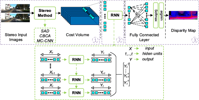

  

  The architecture of the proposed CR-RNN

• 2 The second layer utilizes the RNN network, which has an input comprising a cost vector that includes all disparity values for a given pixel. The inputs of the RNN network (one hidden state), which has an input (X) comprising a cost vector that includes all disparity values for a given pixel. The size of the disparities are dependent on the maximum disparity of the stereo images. The inputs of the RNN network comprised resizing the matching costs according to the time step size of the RNN. The input size of the RNN has to be adjusted to match the Eq. (1) when the time step size changed.

  $$ \mathrm{max\_disp = time\_step\_size \times number\_of\_inputs} $$

  (1)

  By changing the time step size, we determine the input size of the RNN. Costs from stereo method (X) have been resized to [ X₁... X_t−1,X_t] for the different time steps [1... t−1, t]. Each input is given to RNNs with a return sequence structure, and Y_i output is obtained for each X_i input. The return sequential structure provides the interaction of the between the input costs that have sequence structure. The outputs obtained for each time step [ Y₁... Y_t−1,Y_t] are combined and transformed into a single vector.

• 3 In the third layer, the output of the RNN network is applied to a fully connected layer to obtain similarity scores for all possible disparity values. The neuron size of the fully connected layer is equal to the maximum disparity value. Then, the output of the network is given to the Softmax function. In the last step, the smallest value is selected as the corresponding pixel’s disparity value (winner-take-all). Consequently, the resulting architecture of the proposed network is rather simple and shallow in terms of applicability.

4 Results and discussion

4.1 Stereo methods

In this section, details have been given of the existing stereo methods utilized in the proposed structure. In order to obtain the matching cost volume, three different existing popular stereo algorithms that are sum of absolute differences (SAD) [1], cross-based cost aggregation (CBCA) [24], and MC-CNN-Fast [16] are used.

SAD is a simple method for computing the matching cost within a specified area such as a rectangular or square region. When computing the matching cost for a specified area, the given Eq. 2 is used.

$$ C_{\text{SAD}}(p,d) = \sum_{q \epsilon N_{p}} |I^{L}(q) - I^{R}(q-d) | $$

(2)

In Eq. 2, I^L and I^R represent the left and right stereo image pairs, respectively, and d is the disparity value.

Cross-based cost aggregation is an adaptive window selection method that allows each pixel to determine an area to collect only from the pixels within the boundaries of the same object. While determining this adaptive window, a local area is created around each location consisting of pixels with similar image density values. This window is created in two steps. In the first step, it defines the local support zone by creating an upright cross for each pixel. In the second step, borders are determined by looking at the neighborhoods between horizontal pixels for each pixel in this upright cross that created for each pixel.

Proposed structures in MC-CNN [16] are used in this work for both training and testing phases of the proposed structure. We utilized the fast architecture for the stereo method stage of the proposed method to both train and test the CR-RNN network. We selected the fast method for training due to the lower parameter size compared to accurate structure. The accurate architecture is utilized only for the testing of CR-RNN.

4.2 Performance measures

In this work, results are analyzed with both quantitative and qualitative comparisons. For quantitative comparisons, three different metrics were used as the percentage of bad matching pixels (B) [1], endpoint error (EPE) [39], and global difference (GD) [40]. The pixel error rates for different threshold values such as 5, 4, 3, and 2 of B values given in the tables throughout the article. B and EPE are global error measures used to evaluate the entire disparity map. EPE measures errors in the depth information in terms of pixel distances. B, however, rates the number of errors and the total number of pixels. As a result, EPE highlights the weight of major local errors within the total error. EPE is defined in [39] as given in Eq. 3.

$$ E_{\text{EPE}} = \frac{1}{N} \sum_{i \in \Omega}{|y^{i}_{p} - y^{i}_{g}|}, $$

(3)

where y_g is the ground truth disparity value, y_p is the predicted disparity value, and N is the number of pixels in Ω that represents pixels with a disparity value.

The GD measure is used to examine errors that occur at different depths. This criterion is especially important for autonomous systems. Autonomous systems using depth information require the high accuracy of close objects for anti-collision systems, while the distant objects are important for route determination.

The global difference is a distance-aware metric and is designed to measure the error between the ground truth depth value and the disparity estimation. The distance awareness is computed using the depth information obtained using disparity, focal length, and baseline of stereo cameras. The depth map is divided into K points along the depth axis, and the measuring range R_k for each sampled depth point k is defined as [k−r,k+r]. Also, unlike EPE and the percentage of bad matching pixels, the distance awareness curve is drawn using the absolute relative difference (ARD) to distinguish the deviation of disparity in all possible depth values. The ARD is defined as in Eq. 4.

$$ \text{ARD}_{k} = {\frac{1}{N_{R_{k}}} \sum_{y_{g} \in R_{k}}{\frac{|y_{p} -y_{g}|}{y_{g}}} } $$

(4)

where y_g is the ground truth disparity value, y_p is the predicted disparity value, and $N_{R_{k}}$ is the number of pixels in R_k. The global difference (GD) metric was obtained by summing the ARD values at each sample k points as in Eq. 5.

$$ \text{GD} = {\frac{1}{K} \sum_{k \in K}{\text{ARD}_{k}}} $$

(5)

In B and EPE test metrics, the accuracy calculation is made on the 2-dimensional (2D) plane of disparity maps while in the GD metric, the accuracy calculation is made considering the changes in the depth value in the 3D plane.

We have used different r values for GD value calculations and ARD curves. The value of r was set to 4 and 0.5 for GD calculations and ARD curves, respectively. The value of r was set lower for smoother visualization on ARD curves.

4.3 Dataset and training details

We have trained and evaluated our network models using both KITTI 2012 [41] and KITTI 2015 [42] datasets. These datasets composed rectified outdoor images that can be used on autonomous driving applications captured using stereo cameras. The datasets KITTI 2012 and KITTI 2015 contain 194 and 200 rectified images for training and 195 and 200 rectified images for testing, respectively. Each image in these datasets has a ground truth depth image collected with a laser scanner.

The proposed model was trained by using a weighted cross-entropy loss, and we initialize the parameters of our network using a Xavier normal initializer. Nadam is selected as the optimization algorithm. The values of learning rate, β₁ and β₂ parameters of the Nadam algorithm are set to 0.001, 0.9, and 0.999, respectively. The batch size is 128 for each iteration. The network is trained for 15 epochs on an NVIDIA GTX 2080TI and implemented using TensorFlow framework. The weighted cross-entropy loss function is defined in [17, 21] as given Eq. 6.

$$ \text{loss}(y,y_{g}) = \sum_{y_{i}}{P(y_{i},y_{g}) \cdot \text{log} \frac{e^{y_{i}}}{\sum_{j}{e^{y_{j}}}}}, $$

(6)

where y_g refers to ground truth disparities, and P(y_i,y_g) refers to smooth target distribution, centered around the ground truth y_g. The P(y_i,y_g) is defined as in Eq. 7.

$$ P(y_{i},y_{g})=\left\{\begin{array}{ll} \lambda_{1}, & \ \text{if } |y_{i} - y_{g}| \leq 1 \\ \lambda_{2}, & \ \text{if } 1 < |y_{i} - y_{g}| \leq 2\\ \lambda_{3}, & \ \text{if } 2 < |y_{i} - y_{g}| \leq 3\\ 0, & \ \text{otherwise}. \end{array}\right. $$

(7)

The values of the parameters λ₁,λ₂, and λ₃ are set to 0.5, 0.2, and 0.05, respectively.

Before starting the training phase, the KITTI 2012 and KITTI 2015 datasets were examined to explore the distribution of depth values. The results show that the vast majority of depth values are between 0 and 100 as shown in Fig. 2.

Fig. 2

Disparity histograms of KITTI 2012 and KITTI 2015 training datasets

Because of this distribution, the network learns to produce depth information only in the range of 0−100. As a result, the trained network only generates depth values for 0−100 range. In order to deal with this situation, during the training of the proposed network, we have utilized data augmentation only for the training data. Data augmentation has proven to be a very important technique that enables better learning in deep networks when the data has unbalanced distribution. The data used during the training has been expanded by randomly shifting the input data in the range of max_disparity/2−max_disparity. It is avoided to use of different augmentation techniques in order not to alter the disparity values incorrectly. The disparity distribution on the KITTI 2015 test set at the end of the training with and without the augmentation process is given in Fig. 3 which is filtered with a moving average filter with a width of 5, for better visualization.

Fig. 3

Disparity distribution of the training with augmentation and training without augmentation, on the KITTI 2015 test set

In this study, the resulting proposed network is tested on the online test dataset given on the website of the KITTI 2012 and KITTI 2015 datasets. In order to determine the best parameters and enable faster training and validation processes in the development of the proposed network, the training dataset is split as training, validation, and testing.

Two different split ratios were used to examine the learning capabilities of the proposed structure. The MC-CNN-based stereo method is used to determine the results. Three pixels error ratios are given in Tables 1 and 2 for both split sets.

Table 1 Three pixel test error rates for different split ratios of KITTI 2012 dataset

Table 2 Three pixel test error rates for different split ratios of KITTI 2015 dataset

Tables 1 and 2 show that both of the networks are trained better with the increasing size of the training set. This shows that to get better results, the training dataset must be larger.

For the rest of the paper, we used the 80, 10, and 10% splitting ratios for training, validation, and testing, respectively. Also, if it is not stated that the online test dataset available on the website is used, the test results are obtained by using the test dataset that we divide.

4.4 Parameter optimization

The RNN structure proposed in this work has two main parameters that can be adjusted. The first parameter is the hidden layers of the RNN. This parameter directly changes the RNN structure and affects the parameter size of the model. The second parameter is the time step size of the RNN. This parameter depends on the maximum disparity value which is 192 for both datasets. To select the best parameter values for the model, we applied the leave-one-out approach. Firstly, the proposed architecture has been trained and tested with changing sizes of hidden layers while keeping the time step size constant. After finding the appropriate hidden layers, the optimum value of the time step size was determined by using this hidden layers. Also, the MC-CNN-based stereo method is used in this section to determine the parameters of the structure.

The results are given in Table 3 that are obtained as a result of changing the hidden layers by keeping time step size constant at the value of 2.

Table 3 Network performance values for the changing the hidden layers using a fixed time step number

According to Table 3, the error rate B is decreasing with the increasing number of hidden layers. Therefore, the number of the hidden layers is taken as 256. After fixing the size of hidden layers to 256, training and test procedures were carried out to determine the time step size. The results for different time step size values with the related error metrics are given in Tables 4 and 5 for the KITTI 2012 and KITTI 2015 test datasets, respectively.

Table 4 The performance of the proposed network with different time step size values on KITTI 2012 test dataset

Table 5 The performance of the proposed network with different time step size values on KITTI 2015 test dataset

As can be seen from the Table 4, the number of time steps must be kept low to create a network with lower complexity on the KITTI 2012 dataset. Otherwise, the complexity of the network will increase linearly. Table 5 shows similar results as Table 4 when bad matching pixel errors are considered. In addition, according to the bad matching pixel ratios to achieve better performance, the number of time step value should be selected high. Consequently, the optimum value with respect to network complexity and performance needs to be determined depending on the problem.

In the following sections, quantitative and qualitative comparisons are examined. For the quantitative comparisons, the optimal network structures were used in terms of both performance (CR-RNN _P) and parameter size (CR-RNN _C). In qualitative comparisons, the optimum network structure was used on the basis of performance in order to enable better visualization.

4.5 Quantitative comparisons

In order to show the refinement performance of the proposed network (CR-RNN), three different methods as SAD, CBCA, and MC-CNN-Fast are used as stereo method. In addition, the effectiveness of the refinement has been measured using the MC-CNN-Acrt method which has more performance and a more complex structure.

The quantitative comparisons are carried out for both the parameter settings that give the best performance and minimum parameter size. Table 6 is given for the comparison of parameter sizes of the network structured solutions. SAD- and CBCA-based stereo methods are not included in this table as they are not network-based solutions.

Table 6 Comparison of parameter sizes of Network based methods

According to Table 6, when the total number of parameters is compared, both of the proposed CR-RNN architectures use more parameters than the MC-CNN-Fast structure and fewer parameters than the MC-CNN-Acrt structure.

In Tables 7 and 8, the training and validation results are given for different stereo methods used in the proposed structure. The results includes different pixel error rates, EPE, and GD (%) values for comparison.

Table 7 The comparison of the CR-RNN architectures with respect to original methods in terms of total parameters and different error rates on KITTI 2012 test set

Table 8 The comparison of the CR-RNN architectures with respect to original methods in terms of total parameters and different error rates on KITTI 2015 test set

The proposed CR-RNN architectures decreased the bad matching pixel ratios in all metrics given in tables with respect to the corresponding original methods. Furthermore, the CR-RNN _C performs closer to the MC-CNN-Acrt, while the CR-RNN _P performs much better than the MC-CNN-Acrt. When the EPE and GD values considered, CR-RNN _C and CR-RNN _P show much superior performance compared to both of the MC-CNN networks. These comparisons show that the proposed network structure gives better results in both the disparity maps in the 2D plane and the depth maps in the 3D plane. Also, the SAD + CR-RNN _P and CBCA + CR-RNN _P performs better than the original methods.

The results for the original KITTI 2012 and KITTI 2015 online test datasets are given in Table 9.

Table 9 The comparison of the CR-RNN architectures with respect to original methods in terms of and error rates (%) on KITTI 2012 and KITTI 2015 online test set

As seen in the Table 9, it is observed that the performance in both datasets has been increased significantly. According to the results, our proposed method made an improvement of approximately 15% on average. In addition, there are significant improvements in the KITTI 2012 dataset for all bad pixel rates. Similarly, better performance has been achieved for the background and overall regions of the KITTI 2015 dataset. However, for the MC-CNN result, in the foreground region, it is seen that MC-CNN-Fast results are improved and performance values close to MC-CNN-Acrt are obtained. When given the matching costs obtained from CBCA to our network, it is seen that the results are improved in all cases.

4.6 Qualitative comparisons

For qualitative comparison, both ARD curves on test datasets and disparity maps on online test datasets are used. The comparison of ARD curves on KITTI 2012 and KITTI 2015 test datasets is given in Fig. 4a, b.

Fig. 4

The distance-aware ARD curves on KITTI 2012 and KITTI 2015 test datasets

As shown in the figure, the proposed network structure gives quite low error rates in the 3D plane compared to the other models on both test datasets. With the increase in depth values, MC-CNN architectures perform similarly while the proposed method outperforms these networks.

The other qualitative comparisons are given in Fig. 5. On the left side of the figures, left input images are given from both datasets. In Fig. 5, the changing colors in error maps are scaled linearly between black and white. The black color means low error rates and the white color means high error rates. In Fig. 6 the changing colors in error maps show increasing error rates of disparities from dark blue to light blue, and light red to dark red.

Fig. 5

Disparity and error map results for MC-CNN, CBCA, and CR-RNN on the online KITTI 2012 dataset

Fig. 6

Disparity and error map results for MC-CNN, CBCA, and CR-RNN on the online KITTI 2015 dataset

MC-CNN, CBCA, and the refined results using CR-RNN on the online test benchmark in both dataset are given in the Figs. 5a, b, and 6a, b, respectively. The first row of Fig. 5 shows the left input image and disparity map result from left to right. The second row visualizes the error maps for the above-given disparity maps with respect to the ground truth disparity map. In the third row, the zoomed regions of the error maps are visualized in the same order.

The disparity maps in these figures show that the proposed method improved the smooth transition between horizontal disparity values compared to both MC-CNN model and CBCA models. The disparity maps generated by the proposed method have less noisy regions compared to the other models. Also, it can be clearly seen from the error images that the proposed method performs better on the road surfaces and object boundaries. This result is expected due to the use of the sequential information of RNNs.

When the error maps are considered, it is clear that the proposed method has visual improvements in a wider area. Yet, the reduction in numerical errors is not high, as the proposed network structure cannot correct errors locally in several regions on the disparity map.

5 Conclusion

In this paper, a novel approach has been introduced for enhancing the disparity map by improving the matching costs for stereo images. We have utilized RNN to take advantage of the information between sequential pixels. The proposed network adds a few parameters compared to the well-known method MC-CNN-Fast. In quantitative comparisons, the proposed method increased the performance of the MC-CNN-Fast method in both datasets. The performance of the MC-CNN-Acrt has also been increased considerably in almost all test results. In addition, the success of the proposed network has been shown on the matching costs obtained through conventional methods such as CBCA and SAD. Likewise, the qualitative result makes it more visible of the enhancement of the disparity maps. These results prove that the proposed method can be used to improve disparity values on object boundaries and at the same time low-textured areas like roads. The proposed method has a simple and shallow structure. Hence, it can easily be adapted to methods that give matching costs as outputs.

As future work, it can be considered implementing long short-term memory (LSTM) and gated recurrent unit (GRU)-based modules to further improve the performance.

References

D. Scharstein, R. Szeliski, A taxonomy and evaluation of dense two-frame stereo correspondence algorithms. Int. J. Comput. Vis.47(1), 7–42 (2002).
A. Emlek, M. Peker, K. F. Dilaver, in International Artificial Intelligence and Data Processing Symposium (IDAP). Variable window size for stereo image matching based on edge information (IEEEMalatya, 2017), pp. 1–4.
Q. Yang, Stereo matching using tree filtering. IEEE Trans. Pattern. Anal. Mach. Intell.37(4), 834–846 (2015).
C. -S. Huang, Y. -H. Huang, D. -Y. Chan, J. -F. Yang, Shape-reserved stereo matching with segment-based cost aggregation and dual-path refinement. EURASIP J. Image Video Process.2020:, 38 (2020).
X. Huang, Y. -J. Zhang, An o(1) disparity refinement method for stereo matching. Pattern Recog.55:, 198–206 (2016). https://doi.org/10.1016/j.patcog.2016.01.025.
M. Poggi, F. Tosi, S. Mattoccia, Learning a confidence measure in the disparity domain from o(1) features. Comp. Vision Image Underst.193:, 102905 (2020). https://doi.org/10.1016/j.cviu.2020.102905.
J. Redmon, S. Divvala, R. Girshick, A. Farhadi, in Conference on Computer Vision and Pattern Recognition (CVPR). You only look once: unified, real-time object detection (IEEELas Vegas, 2016), pp. 779–788.
H. Yang, B. Fan, L. Guo, Anchor-free object detection with mask attention. EURASIP J. Image Video Process.2020:, 29 (2020).
H. Zhao, J. Shi, X. Qi, X. Wang, J. Jia, in Conference on Computer Vision and Pattern Recognition (CVPR). Pyramid scene parsing network (IEEEHonolulu, 2017), pp. 6230–6239.
A. Dosovitskiy, P. Fischer, E. Ilg, P. Häusser, C. Hazirbas, V. Golkov, P. van der Smagt, D. Cremers, T. Brox, in International Conference on Computer Vision (ICCV). Flownet: learning optical flow with convolutional networks (IEEESantiago, 2015), pp. 2758–2766.
C. Yan, B. Gong, Y. Wei, Y. Gao, Deep multi-view enhancement hashing for image retrieval. IEEE Trans. Pattern. Anal. Mach. Intell., 1–1 (2020). https://doi.org/10.1109/TPAMI.2020.2975798.
C. Yan, B. Shao, H. Zhao, R. Ning, Y. Zhang, F. Xu, 3d room layout estimation from a single rgb image. IEEE Trans. Multimed.22(11), 3014–3024 (2020). https://doi.org/10.1109/TMM.2020.2967645.
C. Yan, Z. Li, Y. Zhang, Y. Liu, X. Ji, Y. Zhang, Depth image denoising using nuclear norm and learning graph model. ACM Trans. Multimedia Comput. Commun. Appl.16(4) (2020). https://doi.org/10.1145/3404374.
J. Chang, Y. Chen, in Conference on Computer Vision and Pattern Recognition. Pyramid stereo matching network (IEEESalt Lake City, 2018), pp. 5410–5418.
G. Yang, H. Zhao, J. Shi, Z. Deng, J. Jia, in Computer Vision – ECCV 2018, ed. by V. Ferrari, M. Hebert, C. Sminchisescu, and Y. Weiss. Segstereo: exploiting semantic information for disparity estimation (SpringerCham, 2018), pp. 660–676.
J. Zbontar, Y. LeCun, in Conference on Computer Vision and Pattern Recognition (CVPR). Computing the stereo matching cost with a convolutional neural network (IEEEBoston, 2015), pp. 1592–1599.
W. Luo, A. G. Schwing, R. Urtasun, in Conference on Computer Vision and Pattern Recognition (CVPR). Efficient deep learning for stereo matching (IEEELas Vegas, 2016), pp. 5695–5703.
P. Brandao, E. Mazomenos, D. Stoyanov, Widening Siamese architectures for stereo matching. Pattern Recogn. Lett.120:, 75–81 (2019).
Z. Chen, X. Sun, L. Wang, Y. Yu, C. Huang, in International Conference on Computer Vision (ICCV). A deep visual correspondence embedding model for stereo matching costs (IEEESantiago, 2015), pp. 972–980.
S. Kim, D. Min, S. Kim, K. Sohn, Unified confidence estimation networks for robust stereo matching. IEEE Trans. Image Process.28(3), 1299–1313 (2019).
A. Shaked, L. Wolf, in Conference on Computer Vision and Pattern Recognition (CVPR). Improved stereo matching with constant highway networks and reflective confidence learning (IEEEHonolulu, 2017), pp. 6901–6910.
H. Hirschmuller, Stereo processing by semiglobal matching and mutual information. IEEE Trans. Pattern. Anal. Mach. Intell.30(2), 328–341 (2008).
N. Mayer, E. Ilg, P. Hässer, P. Fischer, D. Cremers, A. Dosovitskiy, T. Brox, in Conference on Computer Vision and Pattern Recognition (CVPR). A large dataset to train convolutional networks for disparity, optical flow, and scene flow estimation (IEEELas Vegas, 2016), pp. 4040–4048.
K. Zhang, J. Lu, G. Lafruit, Cross-based local stereo matching using orthogonal integral images. IEEE Trans. Circ. Syst. Video Technol.19(7), 1073–1079 (2009). https://doi.org/10.1109/TCSVT.2009.2020478.
A. Emlek, M. Peker, M. K. Yalçin, in 26th Signal Processing and Communications Applications Conference (SIU). Improving the cost-volume based local stereo matching algorithm (IEEEIzmir, 2018), pp. 1–4.
T. Meltzer, C. Yanover, Y. Weiss, in International Conference on Computer Vision (ICCV). Globally optimal solutions for energy minimization in stereo vision using reweighted belief propagation (IEEEBeijing, 2005), pp. 428–435.
V. Kolmogorov, R. Zabih, in Handbook of Mathematical Models in Computer Vision, ed. by N. Paragios, Y. Chen, and O. Faugeras. Graph cut algorithms for binocular stereo with occlusions (SpringerBoston, 2006), pp. 423–437.
R. Spangenberg, T. Langner, S. Adfeldt, R. Rojas, in 2014 IEEE Intelligent Vehicles Symposium Proceedings. Large scale semi-global matching on the cpu, (2014), pp. 195–201. https://doi.org/10.1109/IVS.2014.6856419.
Z. Ma, D. Huang, B. Li, X. Yuan, Asymmetric learning for stereo matching cost computation. IEICE Trans. Inf. Syst.E103.D(10), 2162–2167 (2020). https://doi.org/10.1587/transinf.2020EDP7002.
J. Pang, W. Sun, J. S. Ren, C. Yang, Q. Yan, in International Conference on Computer VisionWorkshops (ICCVW). Cascade residual learning: a two-stage convolutional neural network for stereo matching (IEEEVenice, 2017), pp. 878–886.
A. Kendall, H. Martirosyan, S. Dasgupta, P. Henry, R. Kennedy, A. Bachrach, A. Bry, in International Conference on Computer Vision (ICCV). End-to-end learning of geometry and context for deep stereo regression (IEEEVenice, 2017), pp. 66–75.
Z. Liang, Y. Feng, Y. Guo, H. Liu, W. Chen, L. Qiao, L. Zhou, J. Zhang, in Conference on Computer Vision and Pattern Recognition. Learning for disparity estimation through feature constancy (IEEESalt Lake City, 2018), pp. 2811–2820.
T. P. Nguyen, J. W. Jeon, Wide context learning network for stereo matching. Sig. Process. Image Commun.78:, 263–273 (2019).
M. Poggi, S. Mattoccia, in Proceedings of the BritishMachine Vision Conference (BMVC). Learning from scratch a confidence measure (BMVA PressNew York, 2016), pp. 46–14613.
M. Poggi, S. Mattoccia, in Conference on Computer Vision and Pattern Recognition (CVPR). Learning to predict stereo reliability enforcing local consistency of confidence maps (IEEEHonolulu, 2017), pp. 4541–4550.
F. Cheng, X. He, H. Zhang, Learning to refine depth for robust stereo estimation. Pattern Recog.74:, 122–133 (2018).
Y. Zhong, H. Li, Y. Dai, in Computer Vision – ECCV 2018, ed. by V. Ferrari, M. Hebert, C. Sminchisescu, and Y. Weiss. Open-world stereo video matching with deep rnn (SpringerCham, 2018), pp. 104–119.
M. Gul, M. Bätz, J. Keinert, in Proceedings of the British Machine Vision Conference (BMVC). Pixel-wise confidences for stereo disparities using recurrent neural networks (BMVA PressCardiff, 2019), pp. 1–13.
S. Baker, D. Scharstein, J. P. Lewis, S. Roth, M. J. Black, R. Szeliski, A database and evaluation methodology for optical flow. Int. J. Comput. Vis.92:, 1573–1405 (2011).
G. Yang, X. Song, C. Huang, Z. Deng, J. Shi, B. Zhou, in Conference on Computer Vision and Pattern Recognition (CVPR). Drivingstereo: a large-scale dataset for stereo matching in autonomous driving scenarios (IEEELong Beach, 2019), pp. 899–908.
A. Geiger, P. Lenz, R. Urtasun, in Conference on Computer Vision and Pattern Recognition. Are we ready for autonomous driving? the kitti vision benchmark suite (IEEEProvidence, 2012), pp. 3354–3361.
M. Menze, A. Geiger, in Conference on Computer Vision and Pattern Recognition (CVPR). Object scene flow for autonomous vehicles (IEEEBoston, 2015), pp. 3061–3070.
Acknowledgements
No other acknowledgements.
Funding
This work is supported by Nigde Omer Halisdemir University Research Project Unit under the research grant of MMT 2019/7-BAGEP.
Author information
Authors and Affiliations
Contributions
Authors’ contributions
AE provides data enhancement and codes the total algorithm. Dr. MP designs the total algorithm. AE and MP analyzes the results and wrote the paper. The authors read and approved the final manuscript.
Authors’ information
1. Alper Emlek is currently a Ph.D. student at Nigde Omer Halisdemir University. His research interests include digital image processing, artificial intelligence, and embedded systems.
2. Murat Peker is currently an assistant professor at the Department of Electrical and Electronics Engineering in Nigde Omer Halisdemir University. His research interests include digital signal, image and video processing, embedded systems, and soft computing.
Corresponding author
Ethics declarations
Competing interests
The authors declare that they have no competing interests.
Additional information
Publisher’s Note
Springer Nature remains neutral with regard to jurisdictional claims in published maps and institutional affiliations.
Rights and permissions
Open Access This article is licensed under a Creative Commons Attribution 4.0 International License, which permits use, sharing, adaptation, distribution and reproduction in any medium or format, as long as you give appropriate credit to the original author(s) and the source, provide a link to the Creative Commons licence, and indicate if changes were made. The images or other third party material in this article are included in the article’s Creative Commons licence, unless indicated otherwise in a credit line to the material. If material is not included in the article’s Creative Commons licence and your intended use is not permitted by statutory regulation or exceeds the permitted use, you will need to obtain permission directly from the copyright holder. To view a copy of this licence, visit http://creativecommons.org/licenses/by/4.0/.
About this article
Cite this article
Emlek, A., Peker, M. Refinement of matching costs for stereo disparities using recurrent neural networks. J Image Video Proc. 2021, 11 (2021). https://doi.org/10.1186/s13640-021-00551-9
Received:
Accepted:
Published:
DOI: https://doi.org/10.1186/s13640-021-00551-9