- Research
- Open access
- Published:
Three-dimensional convolutional restricted Boltzmann machine for human behavior recognition from RGB-D video
EURASIP Journal on Image and Video Processing volume 2018, Article number: 120 (2018)
Abstract
This paper provides a novel approach for recognizing human behavior from RGB-D video data. The three-dimensional convolutional restricted Boltzmann machine (3DCRBM) is proposed which can extract features from the raw RGB-D data. In a physical model, the 3DCRBM differs from the restricted Boltzmann machine (RBM) as its weights are shared among all locations in the input and preserving spatial locality. Adjacent frames of the RGB image and the corresponding adjacent frames of the depth image are set as the input of 3DCRBM. Then, multiple 3D convolutional kernels can be applied to these four frames to extract spatio-temporal features. In the experiment of human behavior recognition, the deep belief network (DBN) is established by a layer of 3DCRBM network, convolutional neural network (CNN), and back propagation (BP) network. 3DCRBM is adapted for unsupervised training and getting a feature, while CNN and BP are used for supervised training and classifying the human behavior. The experiment results demonstrate that the correct differentiation rate of 95.7% is achieved, so the effectiveness of our approach could be validated.
1 Introduction
As an important research direction in the field of intelligence, human behavior recognition has gradually attracted people’s attention. At present, human behavior recognition is mainly divided into vision-based recognition and sensor-based identification [1, 2]. The former has been a research hotspot in academia due to its application potential in various fields [3]. The relevantly traditional research methods mainly include the template matching method [4, 5] as well as the state space method [6]. However, these methods are mainly applied to a relatively stable environment, while the accuracy of the light and shadow transformation can be greatly affected under the real complicated situation. Thus, the identification of human behavior characteristics in a real complex environment is the main concern of this study.
In recent years, with the development of deep learning [7], more and more depth models have been introduced with significant effect in various fields, including target detection [8], activity recognition [3, 9], and natural language processing [10]. For example, Ji et al. [11] proposed a convolutional neural network model for video analysis on the basis of the traditional convolutional neural network. This model can decompose the video data into frames and then hard-coded them. After that, multiple convolutional kernel operations are done to extract low-dimensional feature information at the same position in consecutive input frames, and the mean-pooling method will downsample the output features of the convolutions to reduce feature dimensions. This method has got good results in video-based human body recognition. Another method, an unsupervised one, was put forward by Le et al. [12] to directly learn human behavior characteristics from surveillance videos. They designed an independent subspace analysis algorithm (ISA) with the adoption of cascading and convolutional strategies to learn the characteristic information from the data. It has been testified by experiments that the algorithm can obtain higher recognition rates in human behavior recognition. Farabet et al. [13] proposed a method for extracting feature vectors of dense image pixels from multi-scale convolution networks trained by original pixels. Lin et al. [14] decomposed spatio-temporal video sequences in time and space by ASM (approximate string matching) to implement behavior recognition. Ni et al. [15] proposed a multi-level context information depth perception to implement behavior identification. Megavannan et al. [16] made use of depth MHI (motion history image) to capture the motion change processes, and the Hu matrix was used to represent features. Then human behavior recognition can be realized by SVM classifier with the extraction of features. Wang et al. [17] made an action-let ensemble model and applied it to depth image human behavior recognition, and obtained good results. Jalal and Kamal [18] designed a real-time life cycle system and applied it to intelligent home services with the help of the depth silhouette method to realize functions such as action monitoring and behavior identification. Liu et al. [19] used Bayesian networks to estimate the direction of human action. The literature [20] broke the limitation of RGB video through learning the deep video to realize human behavior. The studies above have proved that videos incorporating 3D data features are more complex than the traditional 2D videos. The current recognition rates of human behavior based on 3D video is not high, and its robustness is poor.
In order to achieve recognition of human behavior in RGB-D depth video, this paper is going to present a new 3D convolution-restricted Boltzmann machine model. The model uses multi-dimensional convolutional kernels to extract spatio-temporal feature information from successive RGB and depth images of a video sequence, and it uses the pooling method to reduce the dimension of the feature information. The effectiveness of the algorithm has been verified by the simulation experiment.
2 Basic model
2.1 Restricted Boltzmann machine
The deep belief network (DBN) model was proposed by Hinton et al. as the new life of neural networks [21] in the journal Science in 2006 [22]. This kind of network can extract features with lower dimensionality and higher discrimination from complex high-dimensional input data, and it is structurally compose of multiple restricted Boltzmann machines (RBMs). Roux and Bengio [23] have theoretically confirmed that RBM can fit any types of discrete distribution if the number of elements in the hidden layer is large enough. In recent years, depth algorithms based on RBM have been proved to be effective in image recognition [24], speech recognition [25], text recognition [26], and other fields.
Restricted Boltzmann machine is the most important part of the deep belief network. It is a type of Boltzmann machine with no link between any visible nodes or hidden nodes. Its main advantage is that all visible nodes are independent of others, so do the hidden nodes. Its structure is composed of the visible layer V and the hidden layer H, and there are several nodes in each layer. In the structure, the input layer node represents the evaluation of the object and it is used to stand for the data; the hidden layer represents the state of the evaluated object and it is used to improve the learning ability. Except the link between the two layers, there is no other links between the nodes in each layer. The same layer relies on messages to connect. If there is any change of the message, the state of different layers will be correspondingly changed. The structural characteristics of the restricted Boltzmann machine indicate that the hidden units and the visual ones are respectively independent. The following figure shows the structure and the link weight is represented by W (Fig. 1):

The structure of RBM
2.2 Convolutional neural network
The convolutional neural network (CNN) was first introduced by LeCun [27, 28] as the solution to the problem of excessive parameters caused by the full connection of the input layer during the process of image classification by the neural network. It is a kind of deep neural network with a convolution structure; the structure can reduce the amount of memory occupied by the deep network and the number of parameters of the network and then alleviate the over-fitting problem of the model. The convolutional neural network consists of four layers: an input layer, a convolutional layer, a subsampling layer, and an output layer.
CNN has provided an end-to-end learning model in which the parameters can be trained by the traditional gradient descent method. The trained convolutional neural network can learn the features from the image and complete the extraction and classification of image features. As an important branch in the research of neural networks, the convolutional neural network is characterized by the practicability that the features of each layer can be obtained through the convolution kernel of the shared weight by the local region of the upper layer. Thus, this characteristic makes the convolutional neural network more suitable for the learning and expressing the image features than other neural network methods.
Figure 2 shows the CNN structure. In it, the C layer is a convolution layer. Each neuron in the layer is connected with the local receptive field of the input layer, and it is obtained by a convolution operation of the convolution kernel at the input layer to extract features. The S layer is a subsampling layer. Based on the preservation of the feature information of the convolutional layer, it takes advantage of translation invariance through a pooling operation to reduce the dimension of the feature matrix. The last layer of the CNN is a full-connected layer, it not only transforms the feature information obtained through pooling into a single-dimensional feature vector, but also uses feedback neural network to implement image classification.

CNN Network
Thanks to the shared weights of neurons on a mapping surface in the CNN, the number of network weight parameters and the complexity of network parameter selection are both reduced.
The CNN has become a research focus in the field of image understanding. Its similar weight-sharing network structure with the biological neural networks makes it possible to reduce the complexity of network model as well as the number of weights. This advantage is more obvious when the input of the network is a multi-dimensional image. The image can be directly used as the input of the network, avoiding the complicated feature extraction and data reconstruction processes in the traditional recognition algorithms. The convolutional network is a multi-layer perceptron which specially designs to recognize two-dimensional shapes with its certain invariance to translation, scaling, and other forms of deformation. In a typical CNN structure, the first few layers are usually alternating between the convolutional layer and the downsampling layer, and the last few layers of the network near the output layer are usually fully connected networks. The focus of the training processes of the CNN is to learn the parameters, such as the convolutional kernel parameters of the convolutional layer and the network parameters of the inter-layer connection weight. The prediction process is mainly based on the input image and network parameters to calculate the category label. The keys of the CNN are the network structure (including convolutional layer, downsampling layer, fully connected layer, etc.) and the back propagation algorithms.
3 Methods
The three-dimensional convolutional restricted Boltzmann machine (3DCRBM) is different from the traditional RBM in that it uses a local receptive field to link each output neuron with only a portion of the input neurons. Using the strategy of shared weights, the neuron weights of the same plane are the same, thus reducing the parameters of actual training and the difficulty of network training.
3.1 3D convolution
In the analysis of the video sequence, a plurality of adjacent frames is taken as the input layer data of the 3DCRBM. Since the traditional two-dimensional convolution kernel can only extract the spatial dimension features, the concept of spatio-temporal convolution is proposed. The spatio-temporal convolutions can extract multi-dimensional features of the time and space dimensions through high-dimensional convolution kernels. The volume base layer is linked with a plurality of adjacent frames by means of a high-dimensional convolution kernel, and the motion characteristics of the video sequence are acquired from the space-time high-dimensional space.
Figure 3 shows the differences between two-dimensional convolutions and high-dimensional convolutions. (a) is an ordinary two-dimensional convolution, and (b) the convolution kernels are two-dimensionally convolved in both temporal and spatial dimensions. Use a 2 × 2 high-dimensional convolution strategy. The solid and dashed lines represent the convolution kernels of the two consecutive sets of needles. In each set of convolution kernels, feature mapping weights are shared with each other.

a 2D convolution and b spatial temporal convolution
Because spatio-temporal convolutions share weights when using the same high-dimensional convolution kernel, only a set of features can be extracted in multiple adjacent frames. In order to extract more features in the same set of adjacent frames, in the spatio-temporal convolution process, different high-dimensional convolution kernels are convoluted at the same position in adjacent frames to extract more features. As shown in Fig. 4, in the same position of two adjacent frames, different convolution kernels are used for convolution, so that two different feature maps are obtained.

Multiple convolutional kernel
3.2 3DCRBM algorithm
Like RBM, 3D convolutional RBM is a probabilistic model. We define its energy function as:
where a represents the biased item shared in the visual layer, K represents the number of hidden layers, \( {h}_{ij}^k \) represents the value of the k-th hidden layer. bkdenotes the bias term shared at the k-th hidden layer. ∗ signifies a convolution operation, \( {\tilde{W}}_k \)means that the link weight matrix is flipped, A · B = trATB. According to the principle of thermodynamics, the conditional probability distribution is
where \( \sigma (x)=\frac{1}{1+\exp \left(-x\right)} \). Using formula (2) can calculate the activation probability of the hidden layer nodes.
Since there is no direct link between the visible layer units, it is only associated with the hidden layer h. Therefore, it can be seen that the cells conform to the independent conditional distribution and the condition term is h. The conditional probability distribution is
3.3 Active learning
The attribute tag of the data is the classification information that humans judge through experience and adds data to the data. Video data collected in a real environment is often unlabeled data. These unlabeled data have a low recognition rate in an unsupervised environment, and it is costly to artificially add attribute tags to these data. In response to this problem, the unsupervised active learning is used to improve the recognition rate of the unlabeled data.
A set of unlabeled data is given as X = {x1, …, xn} and the known label classification as Y = {y1, …, yk}.
Select the softmax function as its computed output function. The corresponding loss function J(θ) is
where 1{·} is an indicative formula and the output is 1 or 0. θ = {W, a} The probability that the hypothesis is xi classified as category j is
Calculate the probability P = {p(y1| xi, θ), …, p(yk| xi, θ)} of input xi for each category. If p(yi = j| xi, θ) exceeds the preset threshold δ, then xi is considered to be tagged and classified as yi. For unlabeled data that does not exceed the preset value, you need to calculate the expected gradient length [16] for each action. Its calculation formula is
where ∇J(θ) is the gradient of the loss function
The expected gradient length is a measure of the amount of gradient change for unlabeled data. Since the calculation of the gradient requires a priori label, the expected gradient length can be calculated for the unlabeled data, and the parameter o is selected as the labeled data with the high expected gradient length (EGL) value. The entire network active learning process is shown in Algorithm 1.

4 Networks
On the basis of the 3DCRBM of Chapter 3, a deep belief network is designed to extract feature information of the time and space dimensions. From the physical structure, the network constructed in this paper is logically structured by a layer of 3DCRBM network, convolutional neural network (CNN) network and back propagation (BP) network. 3DCRBM is applied to unsupervised learning of the spatio-temporal characteristics of the video data. CNN and BP are used to provide a supervise training and to determine the type of behavior in the video. The network structure is shown in Fig. 5.

DBN network
3DCRBM is the first layer of the deep structure which includes four layers: the input layer, the convolution layer, the pooling layer, and the output layer. It is shown in Fig. 6.
-
(1)
The input layer is a continuous seven-frame RGB image extracted from the video and a corresponding seven-frame depth image. For the ease of calculation, the RGB image is converted to a grayscale image, then forming a 14 × 320 × 240 input data.
-
(2)
In the C layer, a 21 × 21 × 3 convolution kernel is used to convolve the input layer data. In order to increase the richness of the feature map, two different convolution kernels are used to convolve at the same location, and the C layer finally obtains 10 × 2300 × 220 feature maps.
-
(3)
The S layer is a pooling layer. It uses max-pooling for subsampling. The feature map of the C layer is scaled to improve the robustness of the network for feature patterns. In order to ensure that the output layer can implement a simulated approximation, the S layer of the 3DCRBM sets the scaling factor to 1. The number of feature maps does not change.
-
(4)
The output layer uses convolution kernel of 21 × 21 × 3 to give a convolution operation of feature map after max-pooling, so as to get approximate input of 14 × 320 × 240.
Fig. 6 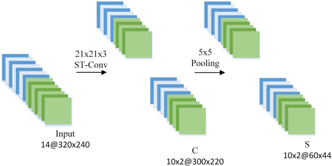
3DCRBM network

After 3DCRBM, a CNN network is set below the deep structure to accept link weights and offset values for unsupervised training 3DCRBM. The input layer and the link weight kij of the C layer and the bias item bj obtained after training 3DCRBM are all initialized and assigned to CNN network. The structure is shown in Fig. 7.
-
1.
The input layer, the C1 layer, and the first two layers of the 3DCRBM assign the convolution kernel values of the trained 3DCRBM to the CNN.
-
2.
The S1 layer, which is a MAX-pool layer, set a scaling factor of 5 to obtain 10 × 2 and 60 × 44 feature maps.
-
3.
The C2 layer uses 11 × 11 × 3 convolution to verify convolution of the two channels. Three different convolution kernels are set up to be convolved to obtain 6 × 6 feature maps, each of which has a size of 50 × 34.
-
4.
The S2 layer is the max-pooling layer. The scaling factor is set to be 2 to scale the C1 layer feature map into 25 × 17. The number of feature maps does not change.
-
5.
In order to unify the dimension in the horizontal and vertical directions of the feature map, C3 obtains a feature map sized 10 × 10 after the operation with a 16 × 8 × 3 convolution kernel. Three different sets of convolution kernels are set up to get 2 × 18 feature maps.
-
6.
The S3 layer is the max-pooling layer. The scale factor is set to be 2 to scale the C1 layer feature map into 5 × 5.
Fig. 7 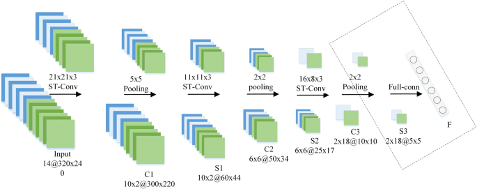
CNN network

After three times of convolutions and subsampling, 2 × 18 sets of feature maps are finally extracted from each seven adjacent frame. These feature maps are expanded into 360 × 1 (= 2 × 18 × 5 × 5 × 1) eigenvectors as the input for the next layer. During the process of spatio-temporal convolution, only 3881 weight parameters need to be trained.
The F layer is the neural network layer and forms the structure in Fig. 7 together with the S3 layer. 360 × 1 eigenvectors are used as the input of back propagation (BP) network, unsupervised learning weights are assigned to BP, and softmax is used as the output function. The entire network is reconstructed according to the error until the error converges.
5 Experimental results and discussions
In order to verify the validity of 3DCRBM, the open source dataset CAD-120 [29] and UTKinect [30] are used as test objects. For each dataset, the effectiveness of our algorithm will be verified through a series of comparative experiments.
5.1 CAD-120 dataset
The CAD120 dataset was collected and published by Jaeyong Sung et al. of CORNEELL University in 2012. The dataset uses Microsoft Kinect as a collector and a total of 120 segments of RGB-D video are captured. Each video clip has a size of 640 × 480 and a duration of 45 s. There are altogether 12 actions in these videos including: washing mouth (A1), brushing teeth (A2), wearing contact lenses (A3), telephoning (A4), drinking (A5), opening a bottle (A6), chopping when cooking (A7), mixing when cooking (A8), chatting in the sofa (A9), lying in the sofa (A10), writing on a whiteboard (A11), and operating the computer (A12). These actions are performed by four volunteers (two men and two women) in five environments (office, kitchen, bedroom, bathroom, and living room). Part of the dataset’s RGB and depth images are shown in Fig. 8.

CAD-120 dataset
The experimental data is classified by K-fold cross-validation (K-fold). The experimental data is divided into K groups and the cross-validation process is repeated K times. During each time, a different part is selected as the test data, and the other K − 1 groups as the training data. Finally, the results of the K experiments are averaged. In this paper, K = 4 is set, that is, video data for each action is divided into four groups, each of which is trained in three groups, and another group is used as the test data repeated four times so that each group of data is taken as a test sample. Finally, the result can be obtained by averaging the test results.
According to the location of different actions, the actions will be assigned to different environments. Figure 9 shows the confusion matrix of 12 types of actions after four layers of cross-validation. From the results, it can be found that the total recognition rate of motion in different environments is 85.7%. In the bathroom environment, the highest rate of motion recognition is 91%. In the living room environment, the minimum recognition rate is 82%. In addition, through experiments it can be seen that the confusion rate of action A5, A6, A7, and A8 is higher, and the motion characteristics of the two groups of actions are similar; therefore, they share a high confusion rate. Moreover, the study has found that the confusion rate is symmetrical, which means, A7 has a higher confusion rate than A8, and vice versa. In order to solve the problem of high confusion, a group of cameras will be probably added to collect the details of actions.

Confusion matrix
Table 1 shows a certain groups of recognition rate raised by some current researchers based on CAD120 dataset. It can be seen that the accuracy rate of our algorithm is relatively high.
5.2 UTKinect dataset
The UTKinect dataset is used as the experimental object to verify the validity of the 3DCRBM algorithm. The dataset has collected 10 actions by 10 different volunteers for a total of 200 video sequences. The 10 actions mainly include the following: walking, sitting down, standing up, picking up something, taking something away, throwing something, pushing, pulling, waving, and clapping. Each volunteer does each movement twice. Since Kinect is used as a video collector, the videos of the RGB and depth channels will be captured. The screenshots of some actions are shown in Fig. 10.

UTKinect dataset
This dataset also uses the K-fold cross-validation (K-fold) method to classify the experimental data. Set K = 6, that is, divide the video data of each action into six groups, train five of them at a time, and use another group as test data, and repeat six times so that each group of data is used as a test sample. Table 2 shows the recognition rate of each action. The motion recognition rate is compared with the one in paper [30], and it is found that the average recognition rate of 10 actions of the 3DCRBM method is 92.9%.
6 Conclusion
This paper proposes a DBN deep network composed of 3DCRBM, CNN, and BP as the verification of 3DCRBM network algorithm and the solution to the problem of depth video human behavior recognition. This algorithm extends the traditional RBM algorithms, increases the convolution layer and the pooling layer, and reduces the use of local receptive field sharing weights. The number of weight parameters and the complexity of network can be reduced by 3DCRBM. In addition, the 3DCRBM algorithm uses 3D convolution at the input layer and uses 3D convolution kernel to extract the spatio-temporal features of adjacent frames.
In order to verify the effectiveness of the 3DCRBM algorithm, this paper constructs a DBN deep network structure composed of 3DCRBM, CNN, and BP and applies it to human behavior recognition experiments. The network structure firstly uses 3DCRBM for unsupervised training and extracts spatio-temporal features from RGB-D images. Then, the link weights of the convolutional layer and the pooling layer of the 3DCRBM are assigned to the CNN, and on the basis of supervised training again, there is a CNN and BP network, and the behavior is identified.
In the human behavior recognition experiment, this paper uses the constructed DBN network to identify the behavior of the two open datasets CAD120 and UTKinect, respectively. Among them, the CAD120 dataset obtains 87.5% recognition rate, and the UTKinect dataset obtains 95.3% recognition rate. It is fully proved that the algorithm has a greater improvement in accuracy than the traditional recognition algorithms.
Abbreviations
- 3DCRBM:
-
Three-dimensional convolutional restricted Boltzmann machine
- ASM:
-
Approximate string matching
- BP:
-
Back propagation
- CNN:
-
Convolutional neural network
- DBN:
-
Deep belief network
- EGL:
-
Expected gradient length
- ISA:
-
Independent subspace analysis
- K-fold:
-
K-fold cross-validation
- MHI:
-
Motion history image
- RBM:
-
Restricted Boltzmann machine
References
M. Ermes, J. Parkka, et al., Detection of daily activity and sports with wearable sensors in controlled and uncontrolled condition. IEEE Trans. Inf. Technol. Biomed. 12(1), 20–26 (2008).
E.A. Heinz, K.S. Kunze, M. Gruber, D. Bannach, P. Lukowicz, Using wearable sensors for real-time recognition tasks in games of martial arts-an initial experiment, in Proc. IEEE Symposium on computational intelligence and games, 98–102 (2006).
M. Baccouche, F. Mamalet, C. Wolf, C. Garcia, A. Baskurt, Sequential deep learning for human action recognition, in Proc. Conference on Human Behavior Understanding, 29–39 (2011).
H.S. Badi, S. Hussein, Hand posture and gesture recognition technology. Neural Comput. & Applic. 25(3–4), 871–878 (2014).
R. Benmokhtar, Robust human action recognition scheme based on high-level feature fusion. Multimedia Tools Appl. 69(2), 253–275 (2014).
M.A.Z. Chahooki, N.M. Charkari, Bridging the semantic gap for automatic image annotation by learning the manifold space. Comput. Syst. Sci. Eng. 30(4), 303–316 (2015).
G.E. Hinton, Learning multiple layers of representation. Trends Cogn Sci. 11(10), 428–434 (2007).
A. Krizhevsky, I. Sutskever, G.E. Hinton, ImageNet classification with deep convolutional neural networks. Adv Neural Inf 2, 1097–1105 (2012).
G. Taylor, R. Fergus, Y. LeCun, C. Bregler, Convolutional learning of spatiotemporal features, in Proc. European Conference on Computer Vision, 140–153 (2010).
X. Glorot, A. Bordes, Y. Bengio, Domain adaptation for large-scale sentiment classification: a deep learning approach, in Proc. Twenty-Eight International Conference on Machine Learning 27, 97–110 (2011).
J. Shuiwang, X. Wei, Y. Ming, Y. Kai, 3D convolutional neural networks for human action recognition. IEEE Trans. Pattern Anal. Mach. Intell. 35(1), 221–231 (2013).
Z.W.Y. Le QV, S.Y. Yeung, A.Y. Ng, Learning hierarchical invariant spatio-temporal features for action recognition with independent subspace analysis, in Proc. IEEE Conference on Computer Vision and Pattern Recognition, 3361–3368 (2011).
C. Farabet, C. Couprie, L. Najman, Y. LeCun, Learning hierarchical features for scene labeling. IEEE Trans. Pattern Anal. Mach. Intell. 35(8), 1915–1929 (2013).
Y. Lin, M. Hu, W. Cheng, Y. Hsieh, H. Chen, Human action recognition and retrieval using sole depth information, in Proc. 20th ACM International Conference on Multimedia, 1053–1056 (2012).
B. Ni, Y. Pei, Z. Liang, L. Lin, P. Moulin, Integrating multi-stage depth-induced contextual information for human action recognition and localization, in Proc. IEEE International Conference And Workshop on Automatic Face and Gesture Recognition, 1–8 (2013).
V. Megavannan, B. Agarwal, R. Badu, Human action recognition using depth maps, in Proc. International Conference on Signal Processing and Communicayions, 1–5 (2012).
J. Wang, Z. Liu, Y. Wu, J. Yuan, Learning actionlet ensemble for 3D human action recognition. IEEE Trans. Pattern Anal. Mach. Intell. 36(5), 914–927 (2014).
A. Jalal, S. Kamal, Real-time life logging via a depth silhouette-based human activity recognition system for smart home services, in Proc. IEEE International Conference on Advanced Video and Signal-Based Surveilance, 74–80 (2014).
W. Liu, Y. Zhang, S. Tang, J. Tang, R. Hong, J. Li, Accurate estimation of human body orientation from RGB-D sensors. IEEE Transact Cybernetics 43(5), 1442–1452 (2013).
D. Zhao, L. Li, H. Peng, Q. Luo, Y. Yang, Multiple routes transmitted epidemics on multiplex networks. Phys. Lett. A 378(10), 770–776 (2014).
G.W. Cottrell, New life for neural networks. SCIENCE 313, 454–455 (2006).
G.E. Hinton, R.R. Salakhutdinov, Reducing the dimensionality of data with neural networks. SCIENCE 313, 504–507 (2006).
N. Le Roux, Y. Bengio, Representational power of restricted Boltzmann machines and deep belief networks. Neural Comput. 20(6), 1631–1649 (2008).
Salakhutdinov, R; Larochelle, H, Efficient learning of deep Boltzmann machines, Journal of Machine Learning Research:Proceedings. 9(1), 693–700, 2010.
N. Jaitly, G. Hinton, Learning a better representation of speech sound waves using restricted Boltzmann machines, in Proc. IEEE Conference on Acoustics, Speech and Signal Processing, 5884–5887 (2011).
G. Dahl, D. Yu, L. Deng, et al., Context-dependent pretrained deep neural networks for large vocabulary speech recognition. IEEE Trans Audio Speech Andlanguage Proc 20(1), 30–42 (2012).
Y. LeCun, L. Bottou, Y. Bengio, P. Haffner, Gradient-based learning applied to document recognition, in Proc. IEEE 86(11), 2278–2324 (1998).
Y. LeCun, K. Kavukcuoglu, C. Farabet, Convolutional networks and applications in vision, in Proc. IEEE International Symposium on Circuits and Systems, 253–256 (2010).
J. Sung, C. Ponce, B. Selman, A. Saxena, Unstructured human activity detection from RGBD images, in Proc. IEEE International Conference on Robotics and Automation, 842–849 (2012).
L. Xia, C. Chen, J.K. Aggarwal, View invariant human action recognition using histograms of 3D joints, in Proc. IEEE Computer Society Conference on Computer Vision and Pattern Recognition Workshops, 20–27 (2012).
H.S. Koppula, R. Gupta, A. Saxena, Learning human activities and object affordances from RGB-D videos. Int J Robotics Res 32(8), 951–970 (2013).
R. Gupta, A.Y. Chia, D. Rajan, Human activities recognition using depth images, In Proceedings of the 2013 Acm Multimedia Conference (2013), pp. 283–292.
B. Ni, Y. Pei, P. Moulin, S. Yan, Multilevel depth and image fusion for human activity detection. IEEE Transact Cybern 43(5), 1383–1394 (2013).
X. Yang, Y. Tian, Effective 3D action recognition using EigenJoints. J. Vis. Commun. Image Represent. 25(1), 2–11 (2013).
L. Piyathilaka, S. Kodagoda, Gaussian mixture based HMM for human daily activity recognition using 3d skeleton features, in Proc. IEEE Conference on Industrial Electronics and Applications, 567–572 (2013).
J. Sung, C. Ponce, B. Selman, A. Saxena, Unstructured human activity detection from RGBD images, in Proc. IEEE Conference on Robotics and Automation, 842–849 (2012).
Acknowledgements
Not applicable.
About the Author
Wang Lukun, Ph.D., currently works at the Department of Information Engineering, Taian Campus, Shandong University of Science and Technology. His current research interests include artificial intelligence, image processing and pattern recognition, machine learning, control theory and applications, and sensor networks.
Availability of data and materials
Authors can provide the data.
Funding
The article is supported by the National Natural Science Foundation of Shandong Province (ZR2018BF005), the Scientific Research Foundation of Shandong University of Science and Technology for Recruited Talents (2017RCJJ077), the Shandong Province Higher Educational Science and Technology Program (J17KB167), and the Science and Technology Program of Taian (2017GX0014).
Author information
Authors and Affiliations
Contributions
The research was performed solely by the author. The author read and approved the final manuscript.
Corresponding author
Ethics declarations
Competing interests
The author declares that he have no competing interests.
Publisher’s Note
Springer Nature remains neutral with regard to jurisdictional claims in published maps and institutional affiliations.
Rights and permissions
Open Access This article is distributed under the terms of the Creative Commons Attribution 4.0 International License (http://creativecommons.org/licenses/by/4.0/), which permits unrestricted use, distribution, and reproduction in any medium, provided you give appropriate credit to the original author(s) and the source, provide a link to the Creative Commons license, and indicate if changes were made.
About this article

Cite this article
Wang, L. Three-dimensional convolutional restricted Boltzmann machine for human behavior recognition from RGB-D video. J Image Video Proc. 2018, 120 (2018). https://doi.org/10.1186/s13640-018-0365-8
Received:
Accepted:
Published:
DOI: https://doi.org/10.1186/s13640-018-0365-8