Directional global three-part image decomposition

Abstract

We consider the task of image decomposition, and we introduce a new model coined directional global three-part decomposition (DG3PD) for solving it. As key ingredients of the DG3PD model, we introduce a discrete multi-directional total variation norm and a discrete multi-directional G-norm. Using these novel norms, the proposed discrete DG3PD model can decompose an image into two or three parts. Existing models for image decomposition by Vese and Osher (J. Sci. Comput. 19(1–3):553–572, 2003), by Aujol and Chambolle (Int. J. Comput. Vis. 63(1):85–104, 2005), by Starck et al. (IEEE Trans. Image Process. 14(10):1570–1582, 2005), and by Thai and Gottschlich are included as special cases in the new model. Decomposition of an image by DG3PD results in a cartoon image, a texture image, and a residual image. Advantages of the DG3PD model over existing ones lie in the properties enforced on the cartoon and texture images. The geometric objects in the cartoon image have a very smooth surface and sharp edges. The texture image yields oscillating patterns on a defined scale which are both smooth and sparse. Moreover, the DG3PD method achieves the goal of perfect reconstruction by summation of all components better than the other considered methods. Relevant applications of DG3PD are a novel way of image compression as well as feature extraction for applications such as latent fingerprint processing and optical character recognition.

1 Introduction

Feature extraction, denoising, and image compression are key issues in computer vision and image processing. We address these main tasks based on the paradigm that an image can be regarded as the addition or montage of several meaningful components. Image decomposition methods attempt to model these components by their properties and to recover the individual components using an algorithm. Relevant component images include geometrical objects which have piece-wise constant values or a smooth surface like the characters in Fig. 1 b or components which are filled with an oscillating pattern like the fingerprint in Fig. 1 c.

Fig. 1

The simulated latent fingerprint (a) is composed by adding the fingerprint (c) to image (b) which is a detail from a photo of a printed document. DG3PD decomposition of a obtains a smooth cartoon image u (d) and a smooth and sparse texture image v (e). All positive coefficients of v are visualized as white pixels in f. The region of interest shown in g is estimated from v_bin using morphological operations [57]. Image i is composed from b and h and decomposed by DG3PD into cartoon (j), texture (k), and residual (l)

Based on these observations, we define the following goals: Goal 1: the cartoon component u contains only geometrical objects with a very smooth surface, sharp boundaries, and no texture. Goal 2: the texture component v contains only geometrical objects with oscillating patterns and v shall be both smooth and sparse. Goal 2: three-part decomposition and reconstruction f=u+v+ε.

How does achieving these goals serve the tasks of feature extraction, denoising, and compression?

Extremely efficient representations of the cartoon image u and texture image v exist. These two component images are highly compressible as discussed with full details in Section 7.3. Depending on the application, u or v or both can be considered as feature images. For the application to latent fingerprints, we are especially interested in the texture image v as a feature for fingerprint segmentation and all subsequent processing steps. Example results for the very challenging task of latent fingerprint segmentation are given in Section 7.1. In optical character recognition (OCR), pre-processing includes the removal of complex background and the isolation of characters. After three-part decomposition and depending on the scale of the characters, the cartoon image u contains the information of interest for OCR (see Fig. 1 j), and the background is separated into v and ε simultaneously in the minimization procedure. As a consequence of the requirements imposed on u and v, noise and small scale objects are driven into the residual image ε during the decomposition of f. Therefore, the image u+v can be regarded as a denoised version of f and the degree of denoising can be steered by the choice of parameters.

The paper is organized as follows. In Section 2, we begin by describing notation and preliminaries. After having established these prerequisites, we define the DG3PD model in Section 3 and in Section 4; we explain its relation to existing models in the literature for two-part and three-part decomposition. In Section 5, we describe an iterative, numerical algorithm which solves the DG3PD model for practical applications to discrete, two-dimensional images. In Section 6, we perform a detailed comparison of the DG3PD method to state-of-the-art decomposition approaches. Applications of DG3PD, especially feature extraction and image compression, are the topics in Section 7. Discussion and conclusions are given in Section 8. An overview of the algorithm and an additional comparison is given in the Appendix.

2 Notation and preliminaries

For simplification, we use a bold symbol to denote the coordinates of a two-dimensional signal, e.g., x=(x ₁,x ₂),k=[k ₁,k ₂],ω=(ω ₁,ω ₂), and $e^{j {\boldsymbol {\omega }}} = \left [ e^{j \omega _{1}} \,, e^{j \omega _{2}} \right ]$. A two-dimensional image $f[\!{\mathbf {k}}] : \Omega \rightarrow \mathbb {R}_{+}$, the discretization of the continuous version f(x) (i.e. f[ k]=f(x)∣ _x=k∈Ω ), is specified on the lattice:

$$\Omega = \left\{ \left(k_{1} \,, k_{2}\right) \in [ 0 \,, m-1 ] \times [ 0 \,, n-1 ] \subset {\mathbb{N}^{2}_{0}} \right\}. $$

Let X be the Euclidean space whose dimension is given by the size of the lattice Ω, i.e., $X = \mathbb {R}^{|{\Omega }|}$. The 2D discrete Fourier transform $\mathcal {F}$ acting on f[ k] is

$$f[\!{\mathbf{k}}] ~\stackrel{\mathcal{F}}{\longleftrightarrow}~ F(e^{j {\boldsymbol{\omega}}}) = \sum_{{\mathbf{k}} \in \Omega} \,f[\!{\mathbf{k}}] \cdot e^{-j \langle {\mathbf{k}} \,, {\boldsymbol{\omega}} \rangle_{\ell_{2}}}, $$

where ω is defined on the lattice:

$${} \begin{aligned} {\mathcal{I}} &= \left\{ (\omega_{1} \,, \omega_{2}) = \left(\frac{2 \pi n^{\prime}}{n} \,, \frac{2 \pi m^{\prime}}{m} \right) \mid (n^{\prime} \,, m^{\prime}) \in \left[ - \frac{n}{2} \,, \frac{n}{2} \right)\right. \\ &\quad \times\left. \left[ - \frac{m}{2} \,, \frac{m}{2} \right) \subset \mathbb{Z}^{2} \right\} \,, \end{aligned} $$

i.e., ω∈[−π,π]².

Forward and backward difference operators: Given the matrix

$${\mathbf{D}_{\mathbf{m}}} = \left(\begin{array}{ccccc} -1 & 1 & 0 & \ldots & 0 \\ 0 & -1 & 1 & \ldots & 0 \\ \vdots & \vdots & \vdots & \ddots & \vdots \\ 0 & 0 & 0 & \ldots & 1 \\ 1 & 0 & 0 & \ldots & -1 \\ \end{array}\right) \in \mathbb{R}^{m \times m}, $$

the forward and backward difference operators with periodic boundary condition in convolution and matrix forms and their Fourier transform are explained in Table 1.

Table 1 Forward/backward difference with periodic boundary condition in convolution/matrix form and their Fourier transform

Discrete directional derivative: Let $\nabla ^{+} = \left [ \partial _{x}^{+} \,, \partial _{y}^{+} \right ]$ be the discrete forward gradient operator with $\partial _{x}^{+}$ and $\partial _{y}^{+}$ defined in Table 1. The discrete derivative operator following the direction $\overrightarrow {d} = \left [ \cos \frac {\pi l}{L} \,, \sin \frac {\pi l}{L} \right ]^{\mathrm {T}}$ with l=0,…,L−1 is defined as

$$\begin{array}{*{20}l} \partial_{l}^{+} &= \left \langle \overrightarrow{d} \,, \nabla^{+} \right \rangle = \cos \left(\frac{\pi l}{L}\right) \partial_{x}^{+} ~+~ \sin \left(\frac{\pi l}{L}\right) \partial_{y}^{+}. \end{array} $$

Thus, the discrete directional gradient operator is

$$ \nabla_{L}^{+} = \left[ \partial_{l}^{+} \right]_{l \in [0, L-1]}. $$

((1))

2.1 Discrete directional TV norm

The continuous total variation norm has been defined in [1]. Due to the discrete nature of images, we define its discrete version with forward difference operators as

$${\left\|\nabla^{+} {\mathbf{u}}\right\|}_{\ell_{1}} = \sum_{{\mathbf{k}} \in \Omega} \sqrt{\left(\partial_{x}^{+} u[\!{\mathbf{k}}]\right)^{2} + \left(\partial_{y}^{+} u[\!{\mathbf{k}}]\right)^{2} }. $$

We extend it into multi-direction L with the discrete directional gradient operator (1):

$$\begin{aligned} {\left\|\nabla_{L}^{+} {\mathbf{u}}\right\|}_{\ell_{1}} &= \sum_{{\mathbf{k}} \in \Omega} \sqrt{\sum\limits_{l=0}^{L-1} \left(\partial_{l}^{+} u[\!{\mathbf{k}}]\right)^{2}} \\&= {\left\|\sqrt{\sum\limits_{l=0}^{L-1} \left(\cos \frac{\pi l}{L} {\mathbf{u}} {\mathbf{D}_{\mathbf{n}}^{\text{T}}} + \sin \frac{\pi l}{L} {\mathbf{D}_{\mathbf{m}}} {\mathbf{u}} \right)^{2}}\right\|}_{\ell_{1}}. \end{aligned} $$

The discrete anisotropic total variation norm in a matrix form is

$$ {\left\|\nabla_{L}^{+} {\mathbf{u}}\right\|}_{\ell_{1}} = \sum\limits_{l=0}^{L-1} {\left\| \cos \frac{\pi l}{L} {\mathbf{u}} {\mathbf{D}_{\mathbf{n}}^{\text{T}}} + \sin \frac{\pi l}{L} {\mathbf{D}_{\mathbf{m}}} {\mathbf{u}} \right\|}_{\ell_{1}}. $$

((2))

2.2 Discrete directional G-norm

Discrete G-norm: Meyer [2] has proposed a space G of continuous functions to measure oscillating functions (texture and noise). The discrete version of the G-norm has been introduced by Aujol and Chambolle in [3]. We rewrite it with the matrix form of the forward difference operators as

$${} {\left\|\mathbf{v}\right\|}_{G} = \inf \left\{{\left\|\sqrt{{{\mathbf{g}}_{1}^{2}} + {{\mathbf{g}}_{2}^{2}}} \right\|}_{\ell_{\infty}},{\mathbf{v}} = {\mathbf{g}}_{1} {\mathbf{D}_{\mathbf{n}}^{\text{T}}} + {\mathbf{D}_{\mathbf{m}}} {\mathbf{g}}_{2}, \left[{\mathbf{g}}_{l} \right]_{l \in [1,2]} \in X^{2}\right\}. $$

((3))

Discrete directional G-norm: We extend (3) into multi-directions $S \in \mathbb {N}_{+}$ with the directional difference operator to obtain the discrete directional G-norm as

$${} {\begin{aligned} {\left\|\mathbf{v}\right\|}_{G_{S}} &\,=\, \inf \left\{\vphantom{\left.\underbrace{{\mathbf{v}} = \sum\limits_{s=0}^{S-1} \left[ \cos \frac{\pi s}{S} {\mathbf{g}}_{s} {\mathbf{D}_{\mathbf{n}}^{\text{T}}} + \sin \frac{\pi s}{S} {\mathbf{D}_{\mathbf{m}}} {\mathbf{g}}_{s} \right] }_{\Leftrightarrow~ v[\!{\mathbf{k}}] = \sum\limits_{s=0}^{S-1} \partial_{s}^{+} g_{s} [\!{\mathbf{k}}] \,, \forall {\mathbf{k}} \in \Omega } \,,~ \left[ {\mathbf{g}}_{s} \right]_{s = 0}^{S-1} \in X^{S} \right\}} {\left\|\sqrt{\sum\limits_{s=0}^{S-1} {{\mathbf{g}}_{s}^{2}}} \right\|}_{\ell_{\infty}},\right.\underbrace{{\mathbf{v}} = \sum\limits_{s=0}^{S-1} \left[ \!\cos \frac{\pi s}{S} {\mathbf{g}}_{s} {\mathbf{D}_{\mathbf{n}}^{\text{T}}} + \sin \frac{\pi s}{S} {\mathbf{D}_{\mathbf{m}}} {\mathbf{g}}_{s} \right] }_{\Leftrightarrow~ v[{\mathbf{k}}] = \sum\limits_{s=0}^{S-1} \partial_{s}^{+} g_{s} [{\mathbf{k}}] \,, \forall {\mathbf{k}} \in \Omega } \,, \\ &\qquad \left. \left[ {\mathbf{g}}_{s} \right]_{s = 0}^{S-1} \in X^{S}\vphantom{\left.\underbrace{{\mathbf{v}} = \sum\limits_{s=0}^{S-1} \left[ \cos \frac{\pi s}{S} {\mathbf{g}}_{s} {\mathbf{D}_{\mathbf{n}}^{\text{T}}} + \sin \frac{\pi s}{S} {\mathbf{D}_{\mathbf{m}}} {\mathbf{g}}_{s} \right] }_{\Leftrightarrow~ v[\!{\mathbf{k}}] = \sum\limits_{s=0}^{S-1} \partial_{s}^{+} g_{s} [\!{\mathbf{k}}] \,, \forall {\mathbf{k}} \in \Omega } \,,~ \left[ {\mathbf{g}}_{s} \right]_{s = 0}^{S-1} \in X^{S} \right\}} \right\}. \end{aligned}} $$

((4))

3 DG3PD

We define the DG3PD model for discrete directional three-part decomposition of an image into cartoon, texture, and residual parts as

$${} \begin{aligned} &\min_{({\mathbf{u}}\,,{\mathbf{v}}\,,{\boldsymbol{\epsilon}}) \in X^{3}} \left\{\vphantom{\frac{1}{2}} {\left\|\nabla_{L}^{+} {\mathbf{u}}\right\|}_{\ell_{1}} + \mu_{1} {\left\|\mathbf{v}\right\|}_{G_{S}} + \mu_{2} {\left\|\mathbf{v}\right\|}_{\ell_{1}}\right. \\&\qquad\qquad\left. \text{s.t. } \sup_{(i, l, k) \in \mathcal{K}} {\left|\mathcal{C}_{i,l} \left\{ {\boldsymbol{\epsilon}} \right\} [\!{\mathbf{k}}]\right|} \leq \delta \,,~ {\mathbf{f}} = {\mathbf{u}} + {\mathbf{v}} + {\boldsymbol{\epsilon}} \right\}, \end{aligned} $$

((5))

where $\mathcal {C}$ is the curvelet transform [4, 5] with the index set $\mathcal {K}$. Please note that by setting the parameter δ=0 in (5), we obtain a two-part decomposition which can be considered as a special case of the DG3PD model. Next, we discuss how the DG3PD model relates to existing decomposition models.

4 Related work

In this section, we give an overview of prior work in two-part and three-part image decomposition in chronological order and we explain how it relates to the proposed DG3PD model.

Mumford and Shah: In 1989, Mumford and Shah [6] have proposed piecewise smooth (for image restoration) and piecewise constant (for image segmentation) models by minimizing the energy functional. This approach can be considered as a precursor for subsequent image decomposition models with texture components. However, due to the Hausdorff one-dimensional measure $\mathcal {H}^{1}$ in $\mathbb {R}^{2}$, it poses a challenging or even NP-hard problem in optimization to minimize the Mumford and Shah functional. Later, based on the Mumford and Shah model, Chan and Vese [7] have proposed an active contour for image segmentation which they solved by a level set method [8].

Rudin, Osher, and Fatemi: In 1992, Rudin et al. [1] pioneered image decomposition with a two-part model for denoising.

Meyer: The model defined by Meyer in 2001 [2] for a two-part decomposition in the continuous setting is comprised in the DG3PD model for the special case of L=S=2 and μ ₂=δ=0 in the discrete domain.

Vese and Osher: In 2003, Vese and Osher [9] solved Meyer’s model for two-part decomposition in the continuous setting and they proposed to approximate the L _∞ -norm in the G-norm by the L ₁-norm and to apply the penalty method for reformulating the constraint. For practical application to images, they discretized their solution. This approach is extended in [10].

Aujol and Chambolle: Aujol and Chambolle in 2005 [3] adapted the work by Meyer for discrete two-part decomposition (see (5.49) in [3]), and they used the penalty method for the constraint. Their model is included in the DG3PD model with parameters L=S=2, μ ₁=μ ₂=0 and applying the supremum norm to the wavelet coefficients of the oscillating pattern, i.e., ${\left \|\mathcal {W} \{ \cdot \}\right \|}_{\ell _{\infty }}$, instead of the curvelet coefficients ${\left \| \mathcal {C} \{ \cdot \}\right \|}_{\ell _{\infty }}$ as in the DG3PD model. Moreover, Aujol and Chambolle proposed a model for discrete three-part decomposition (see (6.59) in [3]) which measures texture by the G-norm and noise by the supremum norm of wavelet coefficients and the penalty method for the constraint. Different from Vese and Osher as well as our approach explained later, they describe the G-norm for capturing texture using the indicator function defined on a convex set and they obtain the solution by Chambolle’s projection onto this convex set. Their model is included in the DG3PD model for parameters L=S=2, μ ₂=0 and using wavelets instead of curvelets for the residual as before.

Starck et al.: Starck et al. [11] introduced a model for two-part decomposition based on a dictionary approach. Their basic idea is to choose one appropriate dictionary for piecewise smooth objects (cartoon) and another suitable dictionary for capturing texture parts.

Aujol et al.: In 2006, Aujol et al. [12] proposed a two-part decomposition of an image into a structure component and a texture component using Gabor functions for the texture part.

Gilles: Gilles [13] proposed a three-part image decomposition method in 2007 which is similar to the Aujol-Chambolle model [3], but G-norm is used as a measurement of the residual (or noise) instead of Besov space $\dot {B}^{\infty }_{-1, \infty }$ with a local adaptability property. Their argument is that the more a function is oscillatory, the smaller is the G norm. Then, they propose a new “merged-algorithm” with a combination of a local adaptivity behavior and Besov space.

Maragos and Evangelopoulos: In 2007, Maragos and Evangelopoulos [14] have proposed a two-part decomposition model which relies on energy responses of a bank of 2D Gabor filters for measuring the texture component. They discuss the connection between Meyer’s oscillating functions [2], Gabor filters [15], and AM-FM image modeling [16, 17].

Buades et al.: In 2010, Buades et al. [18] derived a non-linear filter pair for two-part decomposition into cartoon and texture parts. Further models for two-part decomposition are listed in Table 1 of [18].

Maurel et al. and Chikkerur et al.: In 2011, Maurel et al. [19] proposed a decomposition approach which models the texture component by local Fourier atoms. For fingerprint textures, Chikkerur et al. [20] proposed in 2007 the application of local Fourier analysis (or short-time Fourier transform, STFT) for image enhancement. However, the usefulness of local Fourier analysis for capturing texture information depends on and is limited by the level of noise in the corresponding local window, see Figure 2c in [21] for an example in which STFT enhances some regions successfully and fails in other regions.

Ono et al.: In 2014, Ono et al. [22] proposed a cartoon-texture decomposition using the block nuclear norm (an generalized version of [23]) which interprets the texture component as the combination of overlapped and sheared blockwise low-rank matrices in different directions. The underlying assumption is that “texture, in general, is globally dissimilar but locally well patterned.” Similar to our directional G-norm, the shear helps to handle patterns in non-horizontal or vertical. However, their cartoon component still contains some texture and their texture is not highly sparse, i.e., the non-zero coefficients are only due to texture component, see Fig. 4 a and d, respectively. Moreover, they use ℓ ₁ or ℓ ₂ norm for the data-fidelity term. However, according to [2, 24], “oscillatory components do not have small norms in L ₂(Ω) or L ₁(Ω).” In our case, we use the Banach ${\left \|{\mathcal {C}}\{ \cdot \}\right \|}$ which is more suitable than the Banach space $E = B^{-1}_{\infty, \infty }$ in equation (1.3) [3] for measuring small-scale objects, e.g., noise.

$$ \begin{aligned} &\left({\mathbf{u}}^{\ast} \,, {\mathbf{v}}^{\ast} \,, {\boldsymbol{\epsilon}}^{\ast} \,, \left[ \mathbf{g}_{s}^{\ast} \right]_{s=0}^{S-1} \right) = {\arg\min}_{\left({\mathbf{u}} \,, {\mathbf{v}} \,, {\boldsymbol{\epsilon}} \,, \left[ \mathbf{g}_{s} \right]_{s=0}^{S-1} \right) \in X^{S+3} } \left\{ \sum\limits_{l=0}^{L-1} {\left\|\cos\left(\frac{\pi l}{L} \right) {\mathbf{u}} {\mathbf{D}_{\mathbf{n}}^{\text{T}}} + \sin\left(\frac{\pi l}{L} \right) {\mathbf{D}_{\mathbf{m}}} {\mathbf{u}} \right\|}_{\ell_{1}} \right. \\ & + \mu_{1} \sum\limits_{s=0}^{S-1} {\left\|\mathbf{g}_{s}\right\|}_{\ell_{1}} + \mu_{2} {\left\| \mathbf{v}\right\|}_{\ell_{1}} + G^{\ast} \left(\frac{{\boldsymbol{\epsilon}}}{\delta} \right) ~\text{s.t.}~ \left\{ \begin{array}{l} {\mathbf{f}} = {\mathbf{u}} + {\mathbf{v}} + {\boldsymbol{\epsilon}} \\ {\mathbf{v}} = \sum\limits_{s=0}^{S-1} \left[ \cos\left(\frac{\pi s}{S} \right) {\mathbf{g}}_{s} {\mathbf{D}_{\mathbf{n}}^{\text{T}}} + \sin\left(\frac{\pi s}{S} \right) {\mathbf{D}_{\mathbf{m}}} {\mathbf{g}}_{s} \right] \\ \end{array} \right\}. \end{aligned} $$

((6))

G3PD: A model for discrete three-part decomposition of fingerprint images has recently been proposed by Thai and Gottschlich in 2015 [25] with the aim of obtaining a texture image v which serves as a useful feature for estimating the region of interest (ROI). The G3PD model is included in the DG3PD model by choosing L=2 and replacing the directional G-norm in the DG3PD model by the ℓ ₁-norm of curvelet coefficients (multi-scale and multi-orientation decomposition) to capture texture. However, a disadvantage of the ℓ ₁-norm of curvelet coefficients is a tendency to generate the halo effect on the boundary of the texture region due to the scaling factor in curvelet decomposition (see Figure 3d in [25]), whereas the directional G-norm in the DG3PD model is capable to capture oscillating patterns (see [2]) without the halo effect.

Directional total variation and G-norm: In Section 2.1, we introduced the discrete directional total variation norm, and in Section 2.2, we introduced the discrete directional G-norm. Please note the aspect of summation over multiple directions in Eqs. (2) and (4).

The term “directional total variation” has previously been used by Bayram and Kamasak [26, 27] for defining and computing the TV norm in only one specific direction. They have treated the special case of images with one globally dominant direction and addressed those by two-part decomposition and for the purpose denoising. Zhang and Wang [28] proposed an extension of the work by Bayram and Kamasak for denoising images with more than one dominant direction.

5 Solution of the DG3PD model

Now, we present a numerical algorithm for obtaining the solution of the DG3PD model stated in (5). Given δ>0, denote $G^{\ast }\left (\frac {{\boldsymbol {\epsilon }}}{\delta } \right)$ as the indicator function on the feasible convex set A(δ) of (5), i.e.,

$$\begin{aligned} A(\delta) &= \left\{ {\boldsymbol{\epsilon}} \in X \,:~ {\left\|{\mathcal{C}} \left\{ {\boldsymbol{\epsilon}} \right\}\right\|}_{\ell_{\infty}} \leq \delta \right\} \text{ and } G^{\ast}\left(\frac{{\boldsymbol{\epsilon}}}{\delta} \right)\\ &= \left\{ \begin{array}{ll} 0 \,, & {\boldsymbol{\epsilon}} \in A(\delta) \\ +\infty \,, &{\boldsymbol{\epsilon}} \notin A(\delta) \end{array}\right. \,. \end{aligned} $$

By analogy with the work of Vese and Osher, we consider the approximation of G-norm with ℓ ₁ norm and the anisotropic version of directional total variation norm. The minimization problem in (5) is rewritten as

To simplify the calculation, we introduce two new variables:

$${} \begin{aligned} \left\{\!\! \begin{array}{l} {\mathbf{r}}_{b} = \cos\left(\frac{\pi b}{L} \right) {\mathbf{u}} {\mathbf{D}_{\mathbf{n}}^{\text{T}}} + \sin\left(\frac{\pi b}{L} \right) {\mathbf{D}_{\mathbf{m}}} {\mathbf{u}} \,,~ b = 0 \,, \ldots \,, L-1, \\ {\mathbf{w}}_{a} = {\mathbf{g}}_{a} \,, a = 0 \,, \ldots \,, S-1 \,. \end{array}\right. \end{aligned} $$

Equation (6) is a constrained minimization problem. The augmented Lagrangian method (ALM) is applied to turn (6) into an unconstrained one as

$$ \begin{aligned} &\min_{\substack{\left({\mathbf{u}} \,, {\mathbf{v}} \,, {\boldsymbol{\epsilon}} \,, \left[{\mathbf{r}}_{l}\right]_{l=0}^{L-1} \,, \left[ {\mathbf{w}}_{s} \right]_{s=0}^{S-1} \,, \left[ {\mathbf{g}}_{s} \right]_{s=0}^{S-1} \right) \in X^{L+2S+3} }} \mathcal{L} \left({\mathbf{u}} \,, {\mathbf{v}} \,, {\boldsymbol{\epsilon}} \,, \left[ {\mathbf{r}}_{l} \right]_{l=0}^{L-1} \,,\right.\\&\left. \left[ {\mathbf{w}}_{s} \right]_{s=0}^{S-1} \,, \left[ {\mathbf{g}}_{s} \right]_{s=0}^{S-1} \;; \left[ \boldsymbol{\lambda}_{\boldsymbol{1} l} \right]_{l=0}^{L-1} \,, \left[ \boldsymbol{\lambda}_{\boldsymbol{2}s} \right]_{s=0}^{S-1} \,, \boldsymbol{\lambda}_{\boldsymbol{3}} \,, \boldsymbol{\lambda}_{\boldsymbol{4}} \right) \,, \end{aligned} $$

((7))

where the Lagrange function is

$${} {\begin{aligned} \mathcal{L} (\cdot \;; \cdot) &= \sum\limits_{l=0}^{L-1} {\left\|{\mathbf{r}}_{l}\right\|}_{\ell_{1}} + \mu_{1} \sum\limits_{s=0}^{S-1} {\left\|{\mathbf{w}}_{s}\right\|}_{\ell_{1}} + \mu_{2} {\left\|{\mathbf{v}}\right\|}_{\ell_{1}} + G^{\ast} \left(\frac{\boldsymbol{\epsilon}}{\delta} \right) \\ & \quad + \frac{\beta_{1}}{2} \sum\limits_{l=0}^{L-1} {\left\|{\mathbf{r}}_{l} - \cos\left(\frac{\pi l}{L} \right) {\mathbf{u}} {\mathbf{D}_{\mathbf{n}}^{\text{T}}} - \sin\left(\frac{\pi l}{L} \right) {\mathbf{D}_{\mathbf{m}}} {\mathbf{u}} \frac{\boldsymbol{\lambda}_{\boldsymbol{1} l}}{\beta_{1}}\right\| }^{2}_{\ell_{2}} \\ & \quad + \frac{\beta_{2}}{2} \sum_{s=0}^{S-1} {\left\|{\mathbf{w}}_{s} - {\mathbf{g}}_{s} + \frac{\boldsymbol{\lambda}_{\boldsymbol{2}s}}{\beta_{2}}\right\|}^{2}_{\ell_{2}} \\ & \quad + \frac{\beta_{3}}{2} {\left\|{\mathbf{v}} - \sum\limits_{s=0}^{S-1} \left[\! \cos\left(\! \frac{\pi s}{S}\! \right) {\mathbf{g}}_{s} {\mathbf{D}_{\mathbf{n}}^{\text{T}}} + \sin\left(\! \frac{\pi s}{S}\! \right) {\mathbf{D}_{\mathbf{m}}} {\mathbf{g}}_{s} \!\right] + \frac{\boldsymbol{\lambda}_{\boldsymbol{3}}}{\beta_{3}}\right\| }^{2}_{\ell_{2}} \\&\quad+ \frac{\beta_{4}}{2} {\left\|\mathbf{f}- {\mathbf{u}} - {\mathbf{v}} - {\boldsymbol{\epsilon}} + \frac{\boldsymbol{\lambda}_{\boldsymbol{4}}}{\beta_{4}}\right\|}_{\ell_{2}}^{2}. \end{aligned}} $$

Due to the minimization problem with multi-variables, we apply the alternating directional method of multipliers to solve (7). Its minimizer is numerically computed through iterations t=1,2,…

$$ \begin{aligned} &{\left({\mathbf{u}}^{(t)} \,, {\mathbf{v}}^{(t)} \,, {\boldsymbol{\epsilon}}^{(t)} \,, \left[ {\mathbf{r}}_{l}^{(t)} \right]_{l=0}^{L-1} \,, \left[ {\mathbf{w}}_{s}^{(t)} \right]_{s=0}^{S-1} \,, \left[ {\mathbf{g}}_{s}^{(t)} \right]_{s=0}^{S-1} \right)} ~=~ \\ &{\arg\min} ~ \mathcal{L} \left({\mathbf{u}} \,, {\mathbf{v}} \,, {\boldsymbol{\epsilon}} \,, \left[ {\mathbf{r}}_{l} \right]_{l=0}^{L-1} \,, \left[ {\mathbf{w}}_{s} \right]_{s=0}^{S-1} \,, \left[ {\mathbf{g}}_{s} \right]_{s=0}^{S-1} \;;\right.\\ &\left. \left[ \boldsymbol{\lambda}_{\boldsymbol{1} l}^{(t-1)} \right]_{l=0}^{L-1} \,, \left[ \boldsymbol{\lambda}_{\boldsymbol{2}s}^{(t-1)} \right]_{s=0}^{S-1} \,, \boldsymbol{\lambda}_{\mathbf{3}}^{(t-1)} \,, \boldsymbol{\lambda}_{\mathbf{4}}^{(t-1)} \right) \end{aligned} $$

((8))

and the Lagrange multipliers are updated after every step t with a rate γ. We initialize ${\mathbf {u}}^{(0)} = {\mathbf {f}} \,, {\mathbf {v}}^{(0)} = {\boldsymbol {\epsilon }}^{(0)} = \left [ {\mathbf {r}}_{l}^{(0)} \right ]_{l=0}^{L-1} = \left [ {\mathbf {w}}_{s}^{(0)} \right ]_{s=0}^{S-1} = \left [ {\mathbf {g}}_{s}^{(0)} \right ]_{s=0}^{S-1} = \left [\boldsymbol {\lambda }_{\mathbf {1}l}^{(0)}\right ]_{l=0}^{L-1} = \left [\boldsymbol {\lambda }_{\mathbf {2}a}^{(0)}\right ]_{a=0}^{S-1} = \boldsymbol {\lambda }_{\mathbf {3}}^{(0)} = \boldsymbol {\lambda }_{\mathbf {4}}^{(0)} =\boldsymbol {0}$.In each iteration, we first solve the following six subproblems in the listed order and then we update the four Lagrange multipliers:

The “ $\boldsymbol {\left [ {\mathbf {r}}_{l} \right ]_{l=0}^{L-1}}$-problem”: Fix u, v, ε, $\left [ {\mathbf {w}}_{s} \right ]_{s=0}^{S-1}$, $\left [ {\mathbf {g}}_{s} \right ]_{s=0}^{S-1}$ and

$$ \begin{aligned} &\min_{\substack{\left[ {\mathbf{r}}_{l} \right]_{l=0}^{L-1} \in X^{L}}} \left\{ \sum\limits_{l=0}^{L-1} {\left\|{\mathbf{r}}_{l} \right\|}_{\ell_{1}} + \frac{\beta_{1}}{2} \sum\limits_{l=0}^{L-1} \left\|{\mathbf{r}}_{l} - \cos\left(\frac{\pi l}{L} \right) {\mathbf{u}} {\mathbf{D}_{\mathbf{n}}^{\text{T}}}\right.\right. \\&\qquad\qquad \left.\left. - \sin\left(\frac{\pi l}{L} \right) {\mathbf{D}_{\mathbf{m}}} {\mathbf{u}} + \frac{\boldsymbol{\lambda}_{\boldsymbol{1} l}}{\beta_{1}} \right\|^{2}_{\ell_{2}} \right\} \end{aligned} $$

((9))

Due to its separability, we consider the problem at b=0,…,L−1. The solution of (9) is

$${} {\begin{aligned} {\mathbf{r}}_{b}^{\ast} ~=~ \text{Shrink} \left(\cos\left(\frac{\pi b}{L} \right) {\mathbf{u}} {\mathbf{D}_{\mathbf{n}}^{\text{T}}} + \sin\left(\frac{\pi b}{L} \right) {\mathbf{D}_{\mathbf{m}}} {\mathbf{u}} - \frac{\boldsymbol{\lambda}_{\boldsymbol{1} b}}{\beta_{1}} \,, \frac{1}{\beta_{1}} \right). \end{aligned}} $$

The operator Shrink(·,·) is defined in [25].

The “ $\boldsymbol {\left [ {\mathbf {w}}_{s} \right ]_{s=0}^{S-1}}$-problem”: Fix u, v, ε, $\left [ {\mathbf {r}}_{l} \right ]_{l=0}^{L-1}$, $\left [ {\mathbf {g}}_{s} \right ]_{s=0}^{S-1}$ and

$${} \min_{\substack{ \left[ {\mathbf{w}}_{s} \right]_{s=0}^{S-1} \in X^{S} }} \left\{ \mu_{1} \sum\limits_{s=0}^{S-1} {\left\|{\mathbf{w}}_{s}\right\|}_{\ell_{1}} + \frac{\beta_{2}}{2} \sum\limits_{s=0}^{S-1} {\left\|{\mathbf{w}}_{s} - {\mathbf{g}}_{s} + \frac{\boldsymbol{\lambda}_{\boldsymbol{2}s}}{\beta_{2}}\right\|}^{2}_{\ell_{2}} \right\} $$

((10))

Similarly, the solution of (10) for each separable problem a=0,…,S−1 is

$$ {\mathbf{w}}_{a}^{\ast} ~=~ \text{Shrink} \left(\underbrace{{\mathbf{g}}_{a} - \frac{\boldsymbol{\lambda}_{\boldsymbol{2}a}}{\beta_{2}} }_{:=~ {\mathbf{t}}_{{\mathbf{w}}_{a}}} \,, \frac{\mu_{1}}{\beta_{2}} \right). $$

((11))

The “ $\boldsymbol {\left [ {\mathbf {g}}_{s} \right ]_{s=0}^{S-1}}$-problem”: Fix u, v, ε, $\left [ {\mathbf {r}}_{l} \right ]_{l=0}^{L-1}$, $\left [ {\mathbf {w}}_{s} \right ]_{s=0}^{S-1}$ and

$${} {\begin{aligned} & \min_{\substack{\left[{\mathbf{g}}_{s} \right]_{s=0}^{S-1} \in X^{S}}} \left\{ \frac{\beta_{2}}{2} \sum\limits_{s=0}^{S-1} {\left\|{\mathbf{w}}_{s} - {\mathbf{g}}_{s} + \frac{\boldsymbol{\lambda}_{\boldsymbol{2}s}}{\beta_{2}}\right\|}_{\ell_{2}}^{2}+ \frac{\beta_{3}}{2} \left\|{\mathbf{v}} - \sum\limits_{s=0}^{S-1} \left[ \cos\left(\frac{\pi s}{S} \right) {\mathbf{g}}_{s} {\mathbf{D}_{\mathbf{n}}^{\text{T}}} \right.\right.\right. \\&\quad\qquad \left.\left.\left.+ \sin\left(\frac{\pi s}{S} \right) {\mathbf{D}_{\mathbf{m}}} {\mathbf{g}}_{s} \right] + \frac{\boldsymbol{\lambda}_{\boldsymbol{3}}}{\beta_{3}} \right\|_{\ell_{2}}^{2} \right\} \end{aligned}} $$

((12))

For the discrete finite frequency coordinates ${\boldsymbol {\omega }} = [{\boldsymbol {\omega }}_{1} \,, {\boldsymbol {\omega }}_{2}] \in {\mathcal {I}}$, let be $\phantom {\dot {i}\!}{\mathbf {z}} = [{\mathbf {z}_{\mathbf {1}}} \,, {\mathbf {z}_{\mathbf {2}}}] = \left [ e^{j{\boldsymbol {\omega }_{\boldsymbol {1}}}} \,, e^{j{\boldsymbol {\omega }_{\boldsymbol {2}}}} \right ]$. We denote by W _a (z),Λ _2a (z),V(z),G _s (z), and Λ ₃(z) the discrete Fourier transforms of w _a [ k],λ _2a [ k],v[ k],g _s [ k] and λ ₃[ k], respectively. Due to the separability, the solution of (12) is obtained for a=0,…,S−1 as

$$ {\mathbf{g}}_{a}^{\ast} ~=~ \,\text{Re} \left[ \mathcal{F}^{-1} \left\{ \mathcal{A}({\mathbf{z}}) \cdot \mathcal{B} ({\mathbf{z}}) \right\} \right] $$

((13))

with

$${} {\begin{aligned} & \mathcal{A}({\mathbf{z}}) = \left[{\vphantom{\sum\limits_{1}{1}}} \beta_{2} + \beta_{3} \left[ \sin \frac{\pi a}{S} \left({\mathbf{z}}_{\mathbf{1}}^{-1} - 1\right) + \cos \frac{\pi a}{S} \left({\mathbf{z}}_{\mathbf{2}}^{-1} - 1\right) \right]\right. \\& \qquad\quad\!\! \left. \left[ \sin \frac{\pi a}{S} \left({\mathbf{z}_{\mathbf{1}}} - 1\right) + \cos \frac{\pi a}{S} \left({\mathbf{z}_{\mathbf{2}}} - 1\right) \right] \right]^{-1} \,, \\ & \mathcal{B}({\mathbf{z}}) = \beta_{2} \left[ W_{a}({\mathbf{z}}) + \frac{\Lambda_{2a}({\mathbf{z}}) }{\beta_{2}} \right] + \beta_{3} \left[ \sin\left(\frac{\pi a}{S} \right) \left({\mathbf{z}}_{\mathbf{1}}^{-1} -1\right)\right. \\ &\qquad \left. + \cos\left(\frac{\pi a}{S} \right) ({\mathbf{z}}_{\mathbf{2}}^{-1}-1) \right] \times \\ & \left[ V({\mathbf{z}}) - \sum_{s=[0\,,S-1] \backslash \{a\} } \left[ \cos\left(\frac{\pi s}{S} \right) ({\mathbf{z}_{\mathbf{2}}} - 1) + \sin\left(\frac{\pi s}{S} \right) ({\mathbf{z}_{\mathbf{1}}}-1) \right] \right. \\&\left. G_{s}({\mathbf{z}}) + \frac{\Lambda_{3}({\mathbf{z}})}{\beta_{3}}\vphantom{\left[ V({\mathbf{z}}) - \sum_{s=[0\,,S-1] \backslash \{a\} } \left[ \cos\left(\frac{\pi s}{S} \right) ({\mathbf{z}_{\mathbf{2}}} - 1) + \sin\left(\frac{\pi s}{S} \right) ({\mathbf{z}_{\mathbf{1}}}-1) \right] \right.}\right] \,. \end{aligned}} $$

The “ v -problem”: Fix u, ε, $\left [ {\mathbf {r}}_{l} \right ]_{l=0}^{L-1}$, $\left [ {\mathbf {w}}_{s} \right ]_{s=0}^{S-1}$, $\left [ {\mathbf {g}}_{s} \right ]_{s=0}^{S-1}$ and

$${} \begin{aligned} \min_{{\mathbf{v}} \in X} &\left\{ \mu_{2} {\left\|{\mathbf{v}}\right\|}_{\ell_{1}} + \frac{\beta_{3}}{2} \left\|{\mathbf{v}} - \left(\sum\limits_{s=0}^{S-1} \left[ \cos \left(\frac{\pi s}{S} \right) {\mathbf{g}}_{s} {\mathbf{D}_{\mathbf{n}}^{\text{T}}} \right.\right.\right.\right.\\&\qquad \qquad\; + \left.\left.\left.\left.\sin \left(\frac{\pi s}{S} \right) {\mathbf{D}_{\mathbf{m}}} {\mathbf{g}}_{s} \right] - \frac{\boldsymbol{\lambda}_{\boldsymbol{3}}}{\beta_{3}} \right) \right\|^{2}_{\ell_{2}} \right. \\ & \qquad \qquad \; \left. + \frac{\beta_{4}}{2} {\left\|{\mathbf{v}} - \left({\mathbf{f}} - {\mathbf{u}} - {\boldsymbol{\epsilon}} + \frac{\boldsymbol{\lambda}_{\boldsymbol{4}}}{\beta_{4}} \right) \right\|}_{\ell_{2}}^{2} \right\} \end{aligned} $$

((14))

The solution of (14) is defined as

$$ {\mathbf{v}}^{\ast} ~=~ \text{Shrink} \left({\mathbf{t}}_{\mathbf{v}} \,,~ \frac{\mu_{2}}{\beta_{3} + \beta_{4}} \right), $$

((15))

with

$${} {\begin{aligned} & {\mathbf{t}}_{\mathbf{v}} ~:=~ \frac{\beta_{3}}{\beta_{3} + \beta_{4}} \left(\sum\limits_{s=0}^{S-1} \left[ \cos\left(\frac{\pi s}{S} \right) {\mathbf{g}}_{s} {\mathbf{D}_{\mathbf{n}}^{\text{T}}} + \sin\left(\frac{\pi s}{S} \right) {\mathbf{D}_{\mathbf{m}}} {\mathbf{g}}_{s} \right] - \frac{\boldsymbol{\lambda}_{\boldsymbol{3}}}{\beta_{3}} \right) \\&\qquad + \frac{\beta_{4}}{\beta_{3} + \beta_{4}} \left({\mathbf{f}} - {\mathbf{u}} - {\boldsymbol{\epsilon}} + \frac{\boldsymbol{\lambda}_{\boldsymbol{4}}}{\beta_{4}} \right). \end{aligned}} $$

((16))

The “ u -problem”: Fix v, ε, $\left [ {\mathbf {r}}_{l} \right ]_{l=0}^{L-1}$, $\left [ {\mathbf {w}}_{s} \right ]_{s=0}^{S-1}$, $\left [ {\mathbf {g}}_{s} \right ]_{s=0}^{S-1}$ and

$${} {\begin{aligned} &\min_{{\mathbf{u}} \in X} \left\{ \frac{\beta_{1}}{2} \sum\limits_{l=0}^{L-1} {\left\|{\mathbf{r}}_{l} - \cos\left(\frac{\pi l}{L} \right) {\mathbf{u}} {\mathbf{D}_{\mathbf{n}}^{\text{T}}} - \sin\left(\frac{\pi l}{L} \right) {\mathbf{D}_{\mathbf{m}}} {\mathbf{u}} + \frac{\boldsymbol{\lambda}_{\boldsymbol{1} l}}{\beta_{1}} \right\|}^{2}_{\ell_{2}}\right.\\&\qquad +\left. \frac{\beta_{4}}{2} {\left\|\mathbf{f}- {\mathbf{u}} - {\mathbf{v}} - {\boldsymbol{\epsilon}} + \frac{\boldsymbol{\lambda}_{\boldsymbol{4}}}{\beta_{4}} \right\|}_{\ell_{2}}^{2} \right\} \end{aligned}} $$

((17))

We denote $F({\mathbf {z}}) \,, \mathcal {E}({\mathbf {z}}) \,, \Lambda _{4}({\mathbf {z}}) \,, R_{l}({\mathbf {z}})$, and Λ _1l (z) as the discrete Fourier transforms of f[ k],ε[ k],λ ₄[ k],r _l [ k], and λ _1l [ k], respectively. This (17) is solved in the Fourier domain by

$$ {\mathbf{u}}^{\ast} ~=~ \,\text{Re} \left[ \mathcal{F}^{-1} \left\{ \mathcal{X}({\mathbf{z}}) \cdot \mathcal{Y}({\mathbf{z}}) \right\} \right] $$

((18))

with

$${}\begin{aligned} \mathcal{X}({\mathbf{z}}) &= \left[ \beta_{4} + \beta_{1} \sum\limits_{l=0}^{L-1} \left[ \sin\left(\frac{\pi l}{L} \right) \left({\mathbf{z}}_{\mathbf{1}}^{-1} - 1\right) + \cos\left(\frac{\pi l}{L} \right) \left({\mathbf{z}}_{\mathbf{2}}^{-1} -1\right) \right] \left[ \sin\left(\frac{\pi l}{L} \right) ({\mathbf{z}_{\mathbf{1}}} -1) + \cos\left(\frac{\pi l}{L} \right) \left({\mathbf{z}_{\mathbf{2}}} -1\right) \right] \right]^{-1} \,, \\ \mathcal{Y}({\mathbf{z}}) &= \beta_{4} \left[ F({\mathbf{z}}) - V({\mathbf{z}}) - \mathcal{E}({\mathbf{z}}) + \frac{\Lambda_{4}({\mathbf{z}})}{\beta_{4}} \right] + \beta_{1} \sum\limits_{l=0}^{L-1} \left[ \sin \left(\frac{\pi l}{L} \right) \left({\mathbf{z}}_{\mathbf{1}}^{-1}-1\right) + \cos \left(\frac{\pi l}{L} \right) \left({\mathbf{z}}_{\mathbf{2}}^{-1} -1\right) \right] \left[ R_{l}({\mathbf{z}}) + \frac{\Lambda_{1l}({\mathbf{z}})}{\beta_{1}} \right]. \end{aligned} $$

The “ ε -problem”: Fix u, v, $\left [ {\mathbf {r}}_{l} \right ]_{l=0}^{L-1}$, $\left [ {\mathbf {w}}_{s} \right ]_{s=0}^{S-1}$, $\left [ {\mathbf {g}}_{s} \right ]_{s=0}^{S-1}$, and

$$\begin{array}{*{20}l} \min_{{\boldsymbol{\epsilon}} \in X} \left\{ G^{\ast} \left(\frac{\boldsymbol{\epsilon}}{\delta} \right) + \frac{\beta_{4}}{2} {\left\|{\boldsymbol{\epsilon}} - \left({\mathbf{f}} - {\mathbf{u}} - {\mathbf{v}} + \frac{\boldsymbol{\lambda}_{\boldsymbol{4}}}{\beta_{4}} \right)\right\|}^{2}_{\ell_{2}} \right\} \end{array} $$

((19))

Let $\mathcal {C}^{\ast }$ be the inverse curvelet transform [4]. The minimization of (19) is solved by (see [3])

$$\begin{aligned} {\boldsymbol{\epsilon}}^{\ast} &= \left({\mathbf{f}} - {\mathbf{u}} - {\mathbf{v}} + \frac{\boldsymbol{\lambda}_{\boldsymbol{4}}}{\beta_{4}} \right) \\&\quad - \underbrace{\mathcal{C}^{\ast} \left\{ \text{Shrink} \left(\mathcal{C} \left\{ {\mathbf{f}} - {\mathbf{u}} - {\mathbf{v}} + \frac{\boldsymbol{\lambda}_{\boldsymbol{4}}}{\beta_{4}} \right\} \,, \delta \right) \right\} }_{:=~ \text{CST} \left({\mathbf{f}} - {\mathbf{u}} - {\mathbf{v}} + \frac{\boldsymbol{\lambda}_{\boldsymbol{4}}}{\beta_{4}} \,, \delta \right)} \end{aligned} $$

or by the projection method with the component-wise operators

$${\boldsymbol{\epsilon}}^{\ast} = {\mathcal{C}}^{\ast} \left\{ \frac{\delta \, {\mathcal{C}} \left\{ {\mathbf{f}} - {\mathbf{u}} - {\mathbf{v}} + \frac{\boldsymbol{\lambda}_{\boldsymbol{4}}}{\beta_{4}} \right\}} {\max\left(\delta \,,~ {\left|{\mathcal{C}} \left\{ {\mathbf{f}} - {\mathbf{u}} - {\mathbf{v}} + \frac{\boldsymbol{\lambda}_{\boldsymbol{4}}}{\beta_{4}} \right\}\right|} \right)} \right\}. $$

Update Lagrange multipliers $\left (\left [\boldsymbol {\lambda }_{\mathbf {1}l}\right ]_{l=0}^{L-1} \,, \left [\boldsymbol {\lambda }_{\mathbf {2}a}\right ]_{a=0}^{S-1} \,,\boldsymbol {\lambda }_{\boldsymbol {3}}\,, \boldsymbol {\lambda }_{\boldsymbol {4}} \right) \in X^{L+S+2}$:

$$\begin{aligned} \boldsymbol{\lambda}_{\mathbf{1}b}^{(t)} &= \boldsymbol{\lambda}_{\mathbf{1}b}^{(t-1)} ~+~ \gamma \beta_{1} \left(\mathbf{r}_{b} - \cos\left(\frac{\pi b}{L} \right) {\mathbf{u}} {\mathbf{D}_{\mathbf{n}}^{\text{T}}}\right. \\&\quad \left.- \sin\left(\frac{\pi b}{L} \right) {\mathbf{D}_{\mathbf{m}}} {\mathbf{u}} \right) \,, \quad b = 0 \,, \ldots \,, L-1 \\ \boldsymbol{\lambda}_{\mathbf{2}a}^{(t)} &= \boldsymbol{\lambda}_{\mathbf{2}a}^{(t-1)} + \gamma \beta_{2} \left(\mathbf{w}_{a} - \mathbf{g}_{a} \right) \,, \quad a = 0 \,, \ldots \,, S-1 \\ \boldsymbol{\lambda}_{\mathbf{3}}^{(t)} &= \boldsymbol{\lambda}_{\mathbf{3}}^{(t-1)} + \gamma \beta_{3} \left({\mathbf{v}} - \sum\limits_{s=0}^{S-1} \left[ \cos\left(\frac{\pi s}{S} \right) \mathbf{g}_{s} {\mathbf{D}_{\mathbf{n}}^{\text{T}}}\right.\right. \\&\quad+ \left.\left. \sin\left(\frac{\pi s}{S} \right) {\mathbf{D}_{\mathbf{m}}} \mathbf{g}_{s} \right]\vphantom{\left({\mathbf{v}} - \sum\limits_{s=0}^{S-1} \left[ \cos\left(\frac{\pi s}{S} \right) \mathbf{g}_{s} {\mathbf{D}_{\mathbf{n}}^{\text{T}}}\right.\right.}\right) \\ \boldsymbol{\lambda}_{\mathbf{4}}^{(t)} &= \boldsymbol{\lambda}_{\mathbf{4}}^{(t-1)} + \gamma \beta_{4} \left({\mathbf{f}} - {\mathbf{u}} - {\mathbf{v}} - {\boldsymbol{\epsilon}} \right) \end{aligned} $$

Choice of parameters

Due to the ℓ ₁-norms in the minimization problem (7) which corresponds to the shrinkage operator with parameters μ ₁ and μ ₂, these are defined as

$$\begin{array}{@{}rcl@{}} \mu_{1} &=& c_{\mu_{1}} \beta_{2} \cdot \max_{{\mathbf{k}} \in \Omega} \left({\left| t_{{\mathbf{w}}_{a}}[\!{\mathbf{k}}]\right|} \right) \quad \text{and} \quad \\ \mu_{2} &=& c_{\mu_{2}} \left(\beta_{3} + \beta_{4}\right) \cdot \max_{{\mathbf{k}} \in \Omega} \left({\left| t_{\mathbf{v}} [\!{\mathbf{k}}]\right|} \right), \end{array} $$

((20))

where $\phantom {\dot {i}\!}t_{{\mathbf {w}}_{a}} [\!{\mathbf {k}}]$ and t _v [ k] are defined in (11) and (16), respectively. Note that the choice of $c_{\mu _{1}}$ and $c_{\mu _{2}}$ is adapted to specific images.

In order to balance between the smoothing terms and the updated terms for the solutions of the g-problem in (13), the v-problem in (15), and the u-problem in (18), we choose

$$\beta_{2} = c_{2} \beta_{3} \,, \beta_{3} = \frac{\theta}{1 - \theta} \beta_{4}\,,\theta \in (0,1) \text{ and } \beta_{1} = c_{1} \beta_{4}. $$

The choice of δ mainly impacts the smoothness and sparsity of the texture v. The first row of Fig. 2 shows the effect of selecting the threshold δ=0 which corresponds to a two-part decomposition, i.e., the residual image ε=0 in (d). This case also demonstrates the limitation of all two-part decomposition approaches: for this choice of δ, very small scale objects are assigned to the texture image v in Fig. 2 b which is obvious in its binarization v _bin shown in (c). In order to remove these and to yield a smoother and sparser texture v, one can increase the value of δ, say, e.g., by choosing δ=10. The effect of this choice can be seen in the binarized version v _bin in Fig. 2 g and small-scale objects are moved to the residual image ε in (h). Therefore, the value of δ defines the level of the residual ε.

Fig. 2

Visualization of the decomposition results by DG3PD with δ=0 (a–d) and δ=10 (e–h) after 20 iterations. The convergence rates for these decompositions with δ=0 and δ=10 are depicted in Fig. 6 m, i, respectively, which plots the relative error (y-axis) as defined in [25] versus the number of iterations (x-axis). The parameters are $\protect \phantom {\dot {i}\!}\beta _{4} = 0.04 \,, \theta = 0.9 \,, {{c}_{1}} = 1 \,, c_{2} = 1.3 \,, {{c}_{{\mu }_{1}}} = {{c}_{{\mu }_{2}}} = 0.03 \,, \gamma = 1 \,,$ and S=L=9. Error images are illustrated in j after 20 iterations and in k after 60 iterations with δ=10

6 Comparison of DG3PD with prior art

As stated before, the main objective of the DG3PD model is to achieve the following three goals (see Section 1):

• Goal 1: u contains only geometrical objects with a very smooth surface, sharp boundaries, and no texture.

• Goal 2: v contains only objects with sparse oscillating patterns and v shall be both smooth and sparse.

• Goal 3: Perfect reconstruction of f, i.e., f=u+v+ε.

Based on these criteria, we compare the proposed DG3PD model in this section with the state-of-the-art methods using the original Barbara image. We highlight selected regions for an improved conspicuousness of the differences between the considered methods; see Fig. 3:

• Images without noise: Rudin, Osher, and Fatemi (ROF) [1], Vese and Osher (VO) [9], Starck, Elad, and Donoho (SED) [11], and TV Gabor (TVG) by Aujol et al. [12] models.

• Images corrupted by i.i.d. Gaussian noise $\mathcal {N}(0 \,, \sigma)$: the Aujol and Chambolle (AC) model [3].

Fig. 3

The original Barbara image (a) and highlighted details (b, c)

For better visibility of differences between the various models, we show decomposition results for the ROF, VO, SED, TVG, and DG3PD models for two magnified parts of the original image (see Fig. 3 b, c) in Figs. 4 and 5. We observe two main differences between the compared models and the proposed DG3PD model:

• Two-part decomposition instead of three-part decomposition.

  Fig. 4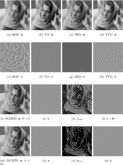

  

  a–p The images in the first row depict the comparison of the cartoon u for different methods in the literature on the original highlighted region (see Fig. 3 c). The images in the second row show their corresponding texture v. Note that the ROF is reported in [12]. The images in the third roware obtained by the DG3PD model with δ=0 and δ=10 in the fourth row (see Fig. 2 for the whole image in these two cases)

  Fig. 5

  

  a–j The images in the first row depict the comparison of the cartoon u for different methods on the original highlighted region (see Fig. 3(b)). The images in the second row show their corresponding texture v

• Quadratic penalty method (QPM) for solving the constrained minimization instead of ALM.

Goal 1: cartoon u. Regarding the cartoon u, we observe that the VO and SED models still contain texture on the scarf (see Fig. 4 b, c, respectively). For the SED, the cartoon u is blurred and there are some small-scale objects under the table (see Fig. 5 c). Comparing all five methods, VO and SED are furthest away from achieving the first goal, whereas ROF and TVG generate better cartoon images in terms of smoother surfaces without texture and sharper boundaries. Recently, Schaeffer and Osher [23] suggested a two-part decomposition approach. Note that the cartoon image by their decomposition which is shown in Figure 7a of [23] also contains texture and does not meet the first goal. The cartoon images produced by the DG3PD method come closest to the first goal, see Fig. 4 i, m and Fig. 5 e.

Goal 2: texture v. Concerning the texture v, among the state-of-the-art methods, the decomposition by the SED model results in the sparsest texture (see Figs. 4 g and 5 h), while the texture images of the ROF, VO, and TVG have more coefficients different from zero. In addition, the texture component obtained by the ROF model also contains some geometry information which should have been assigned to the cartoon component, see Figs. 4 e and 5 f. The DG3PD model yields an even sparser texture than the SED model due to the ${\left \|{\mathbf {v}}\right \|}_{\ell _{1}}$ in the minimization (5), see the binarized versions with threshold “0” for visualization in Fig. 4 o or Fig. 2 g.

Goal 3: reconstruction by summation of all components. Figures 6 and 7 illustrate the effects of QPM and ALM. The decomposition by the ROF model results in a relatively large error (f−u) which contains geometry and texture information; see [9] and Fig. 6 i. In the VO model, the error (f−u−v) is reduced in comparison to the ROF model, but some information still remains in the error image; see Fig. 6 n. In case of the DG3PD model with the ALM-based approach for solving the constrained minimization, the error (f−u−v−ε) is significantly reduced and numerically the error tends to 0 as the number of iterations increases. For a comparison to ROF and VO using the same detail, see Fig. 6 o for a visualization of the error after 20 iterations and (p) after 60 iterations. The error for the whole image after 20 and 60 iterations is displayed in Fig. 2 j, k, respectively. To the best of our knowledge, this effect can be explained by using ALM for solving the constrained minimization instead of QPM. For more details about QPM and ALM, we refer the reader to [29, 30] and Chapter 3 in [31].

Fig. 6

a–l Comparison of QPM and ALM for the ROF, VO, and DG3PD models: The images for ROF and VO models are obtained from [9]. The parameters for the DG3PD model are δ=0 and 20 iterations for the third and 60 for the fourth column, and the other parameters are the same as in Fig. 2. The relative error (y-axis) versus the number of iterations (x-axis) is illustrated in m. The first row shows that the VO and the DG3PD models can achieve good reconstructed images, see b, c, d, in comparison with the original magnified image (a). As mentioned in [9], the error image from the VO model (n) contains much less geometry and texture than the one from the ROF model. However, the error image from our model is much further reduced in comparison to the VO model. After 20 iterations some pieces of information still remain in the error image, see (o). As the number of iterations increases, the error numerically tends to 0; see p after 60 iterations

Fig. 7

The comparison of ALM (a–i) and QPM (j–q) for the DG3PD model with the same parameters and 20 iterations: $\protect \phantom {\dot {i}\!}\beta _{4} = 0.025 \,, \theta = 0.9 \,, c_{1} = 10 \,, c_{2} = 1.3 \,, {c_{{\mu }_{1}}} = {c_{{\mu }_{2}}} = 0.03 \,, \gamma = 1 \,, S = L = 32 \,, \delta = 5$. We observe that the error image of QPM still contains geometry and texture information; see after 20 iterations in p and after 60 in q. Using QPM for constrained minimization is similar to decomposing the original image into four parts, namely cartoon (j), texture (k), residual (m), and error (p). The amount of information in the error image by QPM strongly depends on the choice of parameters (β ₁,β ₂,β ₃,β ₄). However, for ALM, the updated Lagrange multipliers (λ ₁ ,λ ₂,λ ₃,λ ₄) compensate for the choice of (β ₁,β ₂,β ₃,β ₄). Thus, the error numerically tends to 0 as the number of iterations increases, see the error image after 20 iterations in h and after 60 iterations in i

Comparison with Aujol and Chambolle. Figure 8 illustrates a situation in which the image is corrupted by i.i.d. Gaussian noise $\mathcal {N}(0 \,, \sigma)$ with σ=20 and compares DG3PD with the AC model [3] for three-part decomposition. It shows that under “heavy” noise, our DG3PD model still meets the criteria for cartoon u and texture v, i.e.,

• Our cartoon u contains smooth surfaces with sharp edges and no texture; see Fig. 8 e. However, the cartoon u from the AC model is blurry with texture on the scarf; see Fig. 8 a.

  Fig. 8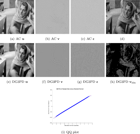

  

  The Barbara image (d) with additive Gaussian white noise (σ=20) is decomposed by the Aujol and Chambolle model (a–c) and the DG3PD model (e–h) with δ=16 and the other parameters are the same as in Fig. 2. Comparing a and e, we observe that the cartoon image u obtained by the DG3PD model (e) has a smoother surface and sharper edges than a. Comparing the texture images v, we note that f is smoother and sparser than b. In order to highlight the sparseness of the DG3PD texture, all positive coefficients are visualized as white pixels in h. For visualization, we add 150 to the value of the residual ε in g. The residual in g still contains some texture, but mainly the Gaussian noise which is obviously shown in the QQ plot (i). There are some differences at the end of the tail in i probably due to the remaining texture and the numerical simulation of Gaussian noise

• Our texture v is sparse and smooth; see Fig. 8 f and its binarization (h). However, the texture from the AC model is not sparse; see Fig. 8 b.

However, there is a limitation for both methods: the noise image ε contains some pieces of information due to the value of δ which defines the level of the noise. Similar to [3], we modify the classical threshold for curvelet coefficients, i.e., $\sigma \sqrt {2 \log {\left |\mathcal {K}\right |}}$, with a weighting parameter η as follows $\delta = \eta \sigma \sqrt {2 \log {\left |\mathcal {K}\right |}}$ and ${\left |\mathcal {K}\right |}$ is total number of curvelet coefficients.

Summary. We observe that the DG3PD method meets all three requirements much more closely than the other methods for images without noise, like the original Barbara image. And in particular, for images with additive noise, the DG3PD method still achieves all three goals as shown in the comparison with Aujol and Chambolle.

7 Applications

Here, we limit ourselves to consider three important applications of the DG3PD method: feature extraction, denoising, and image compression.

7.1 Feature extraction

Depending on the specific field of application, the cartoon or texture, or both can be viewed as feature images. For the application of DG3PD to fingerprints, we are especially interested in the texture image v as a feature for subsequent processing steps like segmentation, orientation field estimation [32] and ridge frequency estimation [15], and fingerprint image enhancement [15, 21]. The first of these processing steps is to separate the foreground from the background [25, 57]. The foreground area (or region of interest) contains the relevant information for a fingerprint comparison. Segmentation is still a challenging problem for latent fingerprints [33] which are very low-quality fingerprints lifted from crime scenes. Both the foreground and background area can contain “noise” on all scales, from small objects or dirt on the surface to written or printed characters (on paper) and large-scale objects like an arc drawn by the forensic examiner. Standard fingerprint segmentation methods cannot cope with this variety of noise, whereas the texture image by decomposition with the DG3PD method crops out to be an excellent feature for estimating the region of interest. Figure 9 depicts a detailed example of the latent fingerprint segmentation by the DG3PD decomposition. In Fig. 10, we show further examples of segmentation results obtained using the texture image extracted by the DG3PD method and morphological postprocessing as described in [25, 57].

Fig. 9

DG3PD decomposition of a latent fingerprint for segmentation (a) with δ=60. b–e The ROI is obtained from the binarized texture v_bin and morphological postprocessing as described in [57]

Fig. 10

Latent fingerprint images from NIST SD27. The boundary of the foreground estimated by the DG3PD method is drawn in yellow (a–d)

7.2 Denoising

The DG3PD model can be used for denoising images with texture because noise and small-scale objects are moved into the residual image ε during the decomposition of f due to the supremum norm of the curvelet coefficients of ε. Therefore, the image f _denoised=u+v can be regarded as a denoised version of f and the degree of denoising can be steered by the choice of parameters, especially δ. For δ=0 which is equal to two-part decomposition, we obtain the original image again. As we increase δ, more noise is driven into ε and thereby removed from f _denoised. Denoising images with texture, in particular with texture parts on different scales, is a relevant problem which we plan to address in future works.

Jung and Kang [34] proposed a variational minimization for vector-valued (color) image decomposition and restoration. Different from our directional total variation, their energy function involves a weighted second-order regularization for the cartoon component also to reduce the staircase effect and to provide image restoration of higher quality. Similar to the Vese-Osher model, they use the L ₂ norm for measuring the residual which is different from our proposed ${\left \|{\mathcal {C}}\{ \cdot \}\right \|}_{\infty }$. Moreover, their reconstructed texture is not sparse due to a lack of the assumption on its sparsity in their minimization model; see Figure 14 b in [34]. In a different view of convex minimization for image reconstruction, Tschumperle [35] proposed a curvature-preserving method for anisotropic smoothing of multi-valued images while preserving natural curvature constraints (or the edges). Then, line integral convolutions are applied for a numerical scheme to this tensor-driven diffusion PDE with two main advantages: namely, it preserves the orientation of thin image structure and the cost of computation is smaller in comparison to the classical explicit scheme. This two-part decomposition scheme is applied for denoising, inpainting, and resizing of vector-valued images.

7.3 Compression

Based on the DG3PD model, we propose a novel approach to image compression. The core idea is to perform image decomposition by the DG3PD method first and subsequently to compress the three component images by three different algorithms, each particularly suited for compressing the specific type of image. This scheme can be used for lossy as well as lossless compression.

7.3.1 Cartoon image compression

As stated in our definition of goals, the cartoon image consists of geometric objects with a very smooth or piecewise constant surface and sharp edges. This special kind of images is highly compressible, and a very effective approach is based on diffusion. Anisotropic diffusion [36] is useful for many purposes in image processing, e.g., fingerprint image enhancement by oriented diffusion filtering [21].

The basic idea of diffusion-based compression is store information for only a few sparse locations which encode the edges of the cartoon image. The surface areas are inpainted using a linear or non-linear diffusion process. Please note that the cartoon image obtained by the DG3PD method is much better suited for this type of compression due to the property of sharper edges between geometric objects in comparison to the cartoon images of the other decomposition approaches. Moreover, some difficulties and drawbacks of diffusion-based compression for arbitrary images do not apply to this special case. In general, it is a challenging question how and where to select locations for diffusion seed points. In our case, this task is easily solvable because of the sharp edges between homogeneous regions in the DG3PD cartoon image. This allows for an extremely sparse selection of locations on corners and edges.

Image compression with edge-enhancing anisotropic diffusion (EED) has been studied by Galic et al. [37] and has been improved by Schmaltz et al. [38]. Compression of cartoon-like images with homogeneous diffusion has been analyzed by Mainberger et al. [39].

A viable alternative to diffusion-based compression of cartoon images is a dictionary-based approach [40] in which the dictionary is optimized for cartoon images. Another very promising possibility to compress the DG3PD cartoon component is the usage of linear splines over adaptive triangulations which has been proposed in the work of Demaret et al. [41].

7.3.2 Texture image compression

Tailor-made solutions are available for texture image compression and especially for compressing oscillating patterns like fingerprints.

Larkin and Fletcher [17] achieved a compression rate of 1:239 for a fingerprint image using amplitude and frequency modulated (AM-FM) functions. They decompose a fingerprint image into four parts, and this idea can be applied to the texture image v obtained by the DG3PD method:

$${\mathbf{v}} \approx \boldsymbol{a} + [ \boldsymbol{b} \cdot \text{cos}(\boldsymbol{\Psi}_{C} + \boldsymbol{\Psi}_{S}) ] $$

Each of the four components is again highly compressible and can be stored with only a few bytes (see Figure 5 in [17]). This is remarkable and we would like to offer another perspective on the AM-FM model. Storing a minutiae template can be viewed as a lossy form of fingerprint compression. The minutiae of a fingerprint are locations where ridges (dark lines) end or bifurcate, and a template stores the locations and directions of these minutiae. Several algorithms have been proposed for reconstructing the orientation field (OF) from a minutia template [42]. The continuous phase Ψ _C can be derived from the unwrapped reconstructed OF and the spiral phase Ψ _S directly constructed from the minutiae template. Choosing appropriate values for a and b leads to a fingerprint image. A survey of further methods for reconstructing fingerprints from their minutiae template is given in [43]. An alternative way of lossy fingerprint image compression is wavelet scalar quantization (WSQ) [44] which has been a compression standard for fingerprints used by the Federal Bureau of Investigation in the USA. See Fig. 11 f–h for application example of WSQ to the texture of the Barbara image.

Fig. 11

The cartoon component u (a) and texture component v (e) of the Barbara image obtained by DG3PD. Images b–d display the reconstruction of u from the 2000, 5000, and 8000 largest wavelet coefficients (from a total of 262,144 coefficients). f–h show the decompressed images after compression of v by WSQ at compression rates between 1:15 and 1:85

A third, very good compression possibility is dictionary learning [40] with optimization of the dictionary for the texture component v. For fingerprint images, this problem has recently been studied by Shao et al. [45].

7.3.3 Residual image compression

For image compression using DG3PD, we propose the following steps in this order: First, image decomposition f=u+v+ε. Second, a tailor-made, lossy, high compression of the cartoon component u and the texture component v. Third, decompressing u and v in order to compute the compression residual image s=f−u _d −v _d , where u _d is the cartoon image and v _d the texture image after decompression. Fourth, compression of s.

In steps two and four, the term “compression” denotes the whole process including coefficient quantization and symbol encoding (see [46] for scalar quantization, Huffman coding, LZ77, LZW, and many other standard techniques).

Let be e _u =u−u _d , the difference between the cartoon component before and after compression, i.e., the compression error, and e _v =v−v _d , then we can rewrite r=f−u _d −v _d =u+v+ε−u _d −v _d =ε+e _u +e _v . Hence, the residual image s computed in step four contains the residual component ε plus the compression errors of the other two components. Now, lossless compression can be achieved by lossless compression of s. If the goal is lossy compression with a certain target quality or target compression rate, this can be achieved by adapting the lossy compression of s accordingly. See Fig. 11 for the effects of different compression rates on the decompressed cartoon u _d and the decompressed texture v _d .

An additional advantage of decompression beginning with u _d , followed by v _d and finally s _d is the fast generation of a preview image which mimics the effects of interlacing. In a scenario with limited bandwidth for data transmission, e.g., sending an image to a mobile phone, the user can be shown a preview based on the compressed, transmitted, and decompressed u image. During the transmission of the compressed v and s, the user can decide whether to continue or abort the transmission.

8 Conclusions

The DG3PD model is a novel method for three-part image decomposition. We have shown that the DG3PD method achieves the goals defined in the introduction much better than other relevant image decomposition approaches. The DG3PD model lays the groundwork for applications such as image compression, denoising, and feature extraction for challenging tasks such as latent fingerprint processing. We follow in the footsteps of Aujol and Chambolle [3] who pioneered three-part decomposition and DG3PD generalizes their approach. We believe that three-part decomposition is the way forward to address many important problems in image processing and computer vision. Buades et al. [18] asked in 2010: “Can images be decomposed into the sum of a geometric part and a textural part?” Our answer to that question is no if an image contains other parts than cartoon and texture, i.e., noise or small-scale objects. Consider, e.g., the noisy Barbara image in Fig. 8 d. If the sum of the cartoon and texture images shall reconstruct the input image f, a two-part decomposition has to assign the noise parts either to the cartoon or to the texture component. In principle, not even the best two-part decomposition model can fully achieve both goals regarding the desired properties of the cartoon and texture component simultaneously. The solution is that noise and small-scale objects which do not belong to the cartoon or texture have to be allotted to a third component.

In our future work, we intend to optimize the DG3PD method for specific applications, especially image compression and latent fingerprint processing. Issues for improvement include the data-driven, automatic parameter selection, and the convergence rate (can the same decomposition be achieved in fewer iterations?) Furthermore, we plan to explore and evaluate specialized compression approaches for cartoon, texture, and residual images.

Additionally, a very interesting application for the residual component can be biometric liveness detection. Recently, Gragnaniello et al. [47] have concluded that high-pass filtering before computing local image descriptors improves the accuracy of their proposed iris liveness detection algorithm. The residual image obtained by DG3PD contains the high-frequency components of the input image. Applications of DG3PD to iris or fingerprint liveness detection [48, 49] are therefore very promising. A survey of local image descriptors for fingerprint, iris, and face liveness detection can be found in [50].

Optimal solutions of transportation problems are the key to compute the earth mover’s distance (EMD) or Wasserstein distance [51]. Recently, Brauer and Lorenz [52] discussed an interesting connection between Meyer’s G-norm and transportation problems. Solving transportation problems for images of dimension 512×512 pixels or larger can be a computationally extremely challenging problem (depending on the number of producers and consumers, and their distribution over the image domain) even for state-of-the-art methods such as the shortlist method [51]. However, in the special case of p=1, the Kantorovich-Rubinstein duality provides a loophole which allows it to avoid solving the associated transportation problem. Based on this property, Brauer and Lorenz [52] proposed a three-part image decomposition with transport norms. Lellmann et al. [53] proposed the use of transport norms for image denosing and two-part image decomposition. We believe that the commonalities between the Vese-Osher model [9], Meyer’s G-norm, and the recently proposed models using transport norms deserve further research.

Moreover, our experiments have shown that the curvelet transform as part of the DG3PD model is very suitable for capturing the residual component in three-part image decomposition in terms of i.i.d. (or weakly correlated) Gaussian (or non-Gaussian) noise. In principle, it is also conceivable to apply the shearlet transform [54], the contourlet transform [55], or the steerable wavelet transform [56] instead of the curvelet transform, and we deem it worth investigating if especially for specific types of images one of these transforms performs considerably better than the others—as part of a DG3PD model with directional total variational norms, directional G-norms, or transport norms.

9 Appendix

Fig. 12

a–f Comparison of decomposition results by the ROF [1], VO [9], SED [11], TVG [12], and DG3PD models. Parameters for DG3PD are $\protect \phantom {\dot {i}\!}\beta _{4} = 0.04 \,, \theta = 0.9 \,, {c_{1}} = 1 \,, c_{2} = 1.3 \,, {{c}_{{\mu }_{1}}} = {{c}_{{\mu }_{2}}} = 0.03 \,, \gamma = 1 \,, S = L = 9$

References

L Rudin, S Osher, E Fatemi, Nonlinear total variation based noise removal algorithms. Physica D. 60(1–4), 259–268 (1992).
Y Meyer, Oscillating Patterns in Image Processing and Nonlinear Evolution Equations (American Mathematical Society, Boston, MA, USA, 2001).
J-F Aujol, A Chambolle, Dual norms and image decomposition models. Int. J. Comput. Vis.63(1), 85–104 (2005).
E Candès, L Demanet, D Donoho, L Ying, Fast discrete curvelet transforms. Multiscale Model. Simul.5(3), 861–899 (2006).
J Ma, G Plonka, The curvelet transform. IEEE Signal Process. Mag.27(2), 118–133 (2010).
D Mumford, J Shah, Optimal approximations by piecewise smooth functions and associated variational problems. Commun. Pure Appl. Math.42(5), 577–685 (1989).
TF Chan, LA Vese, Active contours without edges. IEEE Trans. Image Process.10(2), 266–277 (2001).
S Osher, JA Sethian, Fronts propagating with curvature-dependent speed: algorithms based on Hamilton-Jacobi formulations. J. Comput. Phys.79(1), 12–49 (1988).
LA Vese, S Osher, Modeling textures with total variation minimization and oscillatory patterns in image processing. J. Sci. Comput.19(1–3), 553–572 (2003).
LA Vese, S Osher, Image denoising and decomposition with total variation minimization and oscillatory functions. J. Math. Imaging Vis.20(1–2), 7–18 (2004).
J-L Starck, M Elad, DL Donoho, Image decomposition via the combination of sparse representations and a variational approach. IEEE Trans. Image Process.14(10), 1570–1582 (2005).
J-F Aujol, G Gilboa, T Chan, S Osher, Structure-texture image decomposition—modeling, algorithms, and parameter selection. Int. J. Comput. Vis.67(1), 111–136 (2006).
J Gilles, Noisy image decomposition: a new structure, texture and noise model based on local adaptivity. J. Math. Imaging Vis.28(3), 285–295 (2007).
P Maragos, G Evangelopoulos, in Proc. Int. Symp. Mathematical Morphology. Leveling cartoons, texture energy markers, and image decomposition (Rio de Janeiro, Brazil, 2007), pp. 125–138.
C Gottschlich, Curved-region-based ridge frequency estimation and curved Gabor filters for fingerprint image enhancement. IEEE Trans. Image Process.21(4), 2220–2227 (2012). doi:10.1109/TIP.2011.2170696.
JP Havlicek, DS Harding, AC Bovik, Multidimensional quasi-eigenfunction approximations and multicomponent AM-FM models. IEEE Trans. Image Process.9(2), 227–242 (2000).
KG Larkin, PA Fletcher, A coherent framework for fingerprint analysis: are fingerprints holograms?Optics Express. 15(14), 8667–8677 (2007).
A Buades, TM Le, J-M Morel, LA Vese, Fast cartoon + texture image filters. IEEE Trans. Image Process.19(8), 1978–1986 (2010).
P Maurel, J-F Aujol, G Peyre, Locally parallel texture modeling. SIAM J. Imaging Sci.4(1), 413–447 (2011).
S Chikkerur, A Cartwright, V Govindaraju, Fingerprint image enhancement using STFT analysis. Pattern Recognit.40(1), 198–211 (2007).
C Gottschlich, C-B Schönlieb, Oriented diffusion filtering for enhancing low-quality fingerprint images. IET Biometrics. 1(2), 105–113 (2012).
S Ono, T Miyata, I Yamada, Cartoon-texture image decomposition using blockwise low-rank texture characterization. IEEE Trans. Image Process.23(3), 1128–1142 (2014).
H Schaeffer, S Osher, A low patch-rank interpretation of texture. SIAM J. Imaging Sci.6(1), 226–262 (2013).
JB Garnett, PT Jones, TM Le, LA Vese, Modeling oscillatory components with the homogeneous spaces \(\dot {BMO}^{-\alpha }\) and \(\dot {W}^{-\alpha,p}\). Pure Appl. Math. Q.7(2), 275–318 (2011).
DH Thai, C Gottschlich, Global variational method for fingerprint segmentation by three-part decomposition. IET Biometrics (to appear, doi:10.1049/iet-bmt.2015.0010).
I Bayram, ME Kamasak, in Proc. EUSIPCO. A directional total variation (Bucharest, Romania, 2012), pp. 265–269. http://digital-library.theiet.org/content/journals/10.1049/iet-bmt.2015.0010.
I Bayram, ME Kamasak, Directional total variation. IEEE Signal Process. Lett.19(12), 781–784 (2012). doi:10.1109/LSP.2012.2220349.
H Zhang, Y Wang, Edge adaptive directional total variation. J Eng, 1–2 (2013). http://digital-library.theiet.org/content/journals/10.1049/joe.2013.0116.
R Courant, Variational methods for the solution of problems of equilibrium and vibrations. Bull. Amer. Math. Soc.49(1), 1–23 (1943).
S Boyd, N Parikh, E Chu, B Peleato, J Eckstein, Distributed optimization and statistical learning via the alternating direction method of multipliers. Foundations Trends Mach. Learn.3(1), 1–122 (2011).
M Fortin, R Glowinski, Augmented Lagrangian Methods. Applications to the Numerical Solution of Boundary-value Problems (North-Holland Pub., Amsterdam, Netherlands, 1983).
C Gottschlich, P Mihăilescu, A Munk, Robust orientation field estimation and extrapolation using semilocal line sensors. IEEE Trans. Inform. Forensics Secur.4(4), 802–811 (2009).
A Sankaran, M Vatsa, R Singh, Latent fingerprint matching: a survey. IEEE Access. 2:, 982–1004 (2014).
M Jung, S Kang, Simultaneous cartoon and texture image restoration with higher-order regularization. SIAM J. Imaging Sci.8(1), 721–756 (2015).
D Tschumperlé, Fast anisotropic smoothing of multi-valued images using curvature-preserving PDE’s. Int. J. Comput. Vis.68(1), 65–82 (2006).
J Weickert, Anisotropic Diffusion in Image Processing (Teubner, Stuttgart, Germany, 1998).
I Galic, J Weickert, M Welk, A Bruhn, A Belyaev, H-P Seidel, Image compression with anisotropic diffusion. J. Math. Imaging Vis.31(2–3), 255–269 (2008).
C Schmaltz, P Peter, M Mainberger, F Ebel, J Weickert, A Bruhn, Understanding, optimising, and extending data compression with anisotropic diffusion. Int. J. Comput. Vis.108(3), 222–240 (2014).
M Mainberger, A Bruhn, J Weickert, S Forchhammer, Edge-based compression of cartoon-like images with homogeneous diffusion. Pattern Recognit.44(9), 1859–1873 (2011).
M Elad, M Aharon, Image denoising via sparse and redundant representations over learned dictionaries. IEEE Trans. Image Process.15(12), 3736–3745 (2006).
L Demaret, N Dyn, A Iske, Image compression by linear splines over adaptive triangulations. Signal Process.86(7), 1604–1616 (2006).
L Oehlmann, S Huckemann, C Gottschlich, in Proc. IWBF. Performance evaluation of fingerprint orientation field reconstruction methods (Gjovik, Norway, 2015), pp. 1–6.
C Gottschlich, S Huckemann, Separating the real from the synthetic: minutiae histograms as fingerprints of fingerprints. IET Biometrics. 3(4), 291–301 (2014). doi:10.1049/iet-bmt.2013.0065.
T Hopper, C Brislawn, J Bradley, WSQ gray-scale fingerprint image compression specification. Technical report, Federal Bureau of Investigation (February 1993). http://www.nist.gov/itl/iad/ig/wsq.cfm.
G Shao, Y Wu, A Yong, X Liu, T Guo, Fingerprint compression based on sparse representation. IEEE Trans. Image Process.23(2), 489–501 (2014).
D Salomon, Data Compression, Fourth edition (Springer, London, UK, 2007).
D Gragnaniello, C Sansone, L Verdoliva, Iris liveness detection for mobile devices based on local descriptors. Pattern Recognit. Lett.57:, 81–87 (2015).
C Gottschlich, Convolution comparison pattern: an efficient local image descriptor for fingerprint liveness detection. PLoS ONE. 11(2), 0148552 (2016).
C Gottschlich, E Marasco, AY Yang, B Cukic, in Proc. IJCB. Fingerprint liveness detection based on histograms of invariant gradients (ClearwaterFL, USA, 2014), pp. 1–7.
D Gragnaniello, G Poggi, C Sansone, L Verdoliva, An investigation of local descriptors for biometric spoofing detection. IEEE Trans. Inform. Forensics Secur.10(4), 849–863 (2015).
C Gottschlich, D Schuhmacher, The shortlist method for fast computation of the earth mover’s distance and finding optimal solutions to transportation problems. PLoS ONE. 9(10), 110214 (2014).
C Brauer, D Lorenz, in Proc. SSVM. Cartoon-texture-noise decomposition with transport norms (Lege-Cap FerretFrance, 2015), pp. 142–153.
J Lellmann, D Lorenz, C-B Schönlieb, T Valkonen, Imaging with Kantorovich–Rubinstein discrepancy. SIAM J. Imaging Sci.7(4), 2833–2859 (2014).
(G Kutyniok, D Labate, eds.), Shearlets. Multiscale Analysis for Multivariate Data (Birkhäuser, Boston, MA, USA, 2012).
MN Do, M Vetterli, The contourlet transform: an efficient directional multiresolution image representation. IEEE Trans. Image Process.14(12), 2091–2106 (2005).
M Unser, DVD Ville, Wavelet steerability and the higher-order Riesz transform. IEEE Trans. Image Process.19(3), 636–652 (2010).
DH Thai, S Huckemann, C Gottschlich, Filter design and performance evaluation for fingerprint image segmentation (2015). arXiv:1501.02113 [cs.CV].
Acknowledgements
The authors would like to thank Luminita Vese for her permission to show the images in Figs. 4(b, f), 5(b, g), 6(b, f, j, n, e, i) and 12(a, b). The authors would like to thank Jean-Francois Aujol for his permission to depict the images in Figs. 4(d, h), 5(d, i), 8(a, b, c) and 12(d, h, a, e). The authors would like to thank Jean-Luc Starck for his permission to display the images in Figs. 4(c, g), 5(c, h), and 12(c, g). The authors gratefully acknowledge support by the German Research Foundation (DFG) and the Open Access Publication Funds of the University of Göttingen. D.H. Thai is supported by the National Science Foundation under Grant DMS-1127914 to the Statistical and Applied Mathematical Sciences Institute. C. Gottschlich gratefully acknowledges support by the Felix-Bernstein-Institute for Mathematical Statistics in the Biosciences and the Niedersachsen Vorab of the Volkswagen Foundation.
Author information
Authors and Affiliations
Corresponding author
Additional information
Competing interests
The authors declare that they have no competing interests.
Rights and permissions
Open Access This article is distributed under the terms of the Creative Commons Attribution 4.0 International License(http://creativecommons.org/licenses/by/4.0/), which permits unrestricted use, distribution, and reproduction in any medium, provided you give appropriate credit to the original author(s) and the source, provide a link to the Creative Commons license, and indicate if changes were made.
About this article
Cite this article
Thai, D.H., Gottschlich, C. Directional global three-part image decomposition. J Image Video Proc. 2016, 12 (2016). https://doi.org/10.1186/s13640-016-0110-0
Received:
Accepted:
Published:
DOI: https://doi.org/10.1186/s13640-016-0110-0