A high capacity reversible data hiding through multi-directional gradient prediction, non-linear regression analysis and embedding selection

Abstract

The technique of reversible data hiding enables an original image to be restored from a stego-image with no loss of host information, and it is known as a reversible data hiding algorithm (RDH). Our goal is to design a method to predict pixels effectively, because the more accurate the prediction is, the more concentrated the histogram is, and it minimizes shifting to avoid distortion. In this paper, we propose a new multi-directional gradient prediction method to generate more accurate prediction results. In embedding stage, according to the embedding capacity of information, we generate the best decision based on non-linear regression analysis, which can differentiate between embedding region and non-embedding region to reduce needless shifting. Finally, we utilize the automatic embedding range decision. With sorting by the amount of regional variance, the easier predicted region is prior for embedding, and the quality of the image is improved after embedding. To evaluate the proposed reversible hiding scheme, we compared other methods on different pictures. Results show that the proposed scheme can embed much more data with less distortion.

1 Introduction

Reversible data hiding (RDH) approach has been applied to some sensible and crucial messages, such as medical images, military pictures, criminal site pictures, digital files of rare artworks. These applications are not allowed to have any distortion. Over the past decade, the reversible data hiding techniques have been proposed. It can be divided into spatial domain [1–18] and frequency domain [19, 20]. In the spatial domain, these techniques also can be divided into three classifications: lossless compression, expansion based (EB), and histogram shifting (HS). In recent years, RDH was based on lossless compression [1–4]. These methods utilized storage space for embedding. [3] proposed the least significant bit (LSB) method, which increases compression efficiency by means of change in least bits to act as supplementary information. However, it cannot get a satisfying performance based on the method of lossless compression, because of the capacity embedding increases, more bit change is needed. As a result, distortion is more dramatic. Difference expansion (DE) was first proposed by [5]. This method was divided an image into pixel pairs and each pair to hide a message was used. [6, 7] also proposed a concept of triplets and tetrads DE. [8] first proposed histogram shifting (HS) in 2006. This method makes a histogram statistic from an image. After generating a histogram, the vacancies between the zero point and the peak point are utilized for shifting. It relies heavily on the most frequently found pixel value. As a result, though HS has good image quality, its hiding ability is lower than DE generally. [9] utilized relevant characteristics of neighbor image by dividing an image into N images by sub-sampling to improve the 0 bin performance of the embedding histogram. Luo et al. [10] proposed the median preservation in each group as a reference pixel to generate an improved histogram. As a result, the RDH system is better than Kim et al.’s. [11] proposed an inverse “s” scan method to increases the concentration of the histogram. [12] proposed also another structure of prediction. The author used a rhombus pattern arrangement to split the image into two groups. Furthermore, [13] used the 2-staged checkerboard prediction proposed by himself [14]. Author assumed the hidden data must be embedding in small-capacity of bins and bins − 2, − 1, 0, 1, and 2 should be kept without change, due to all bins are shift necessarily before embedding. Therefore, both the embedding capacity and image quality still much left for improvement to be improved.

Besides mentioned works above [1–14], many other RDH algorithms are also based on histogram shifting method using different techniques, i.e., Qin et al. [15] proposed a prediction-based reversible steganographic scheme based on image inpainting. This method utilizes partial differential equation (PDE) based on CDD model to effectively predict the structure and geometric information of the original image according to select reference pixels. However, its thresholds of the reference pixels are selected by experimental rule and it also has a problem of large amount of the computation complexity. [16] proposed a general framework, which can simply designing the so-called shifting and embedding functions to reduce the amount of distortion when embedding. Their method actually has good effect when the amount of embedding messages is small, but when the amount of embedding messages gets bigger, the distortion will relatively become higher. The use of least square predictor has been proposed to overcome the limitation of the fixed predictors by [17]. It applied least absolute shrinkage and selection operator over normal least square predictor with rhombus-shaped two-stage embedding scheme. Wang et al. [18] proposed a reversible data hiding based on multiple histogram shifting with rate and distortion optimization. Traditional schemes used experimental rule to determine the number of optimal peak and zero bin pairs and their corresponding values. In order to solve this problem, the genetic algorithm (GA) in optimization algorithm is applied to search the nearly optimal zero and peak bins, and to achieve the purpose of increasing capacity and reducing distortion.

On the other hand, in recent years, due to privacy requirement, image owners often encrypt the original content before transferring it to a data manager. The data manager wants to embed other messages in an encrypted image for authentication, even the content of the original image is unknown to him. Therefore, image encryption is a method that protects the contents of the original images for the owners of the images. Generally, there are three roles in the reversible data hiding method on image encryptions, including content owners, data hiders, and receivers. The current encrypted RDH scheme embedding mechanism can be divided into two processes, one is reserving room before encryption (RRBE) [21–23], and the other is vacating room after encryption (VRAE) [24–28]. In general, the scheme of the RRBE process has better hiding power and recovery ability than the scheme of the VRAE process. But, VRAE process scheme does not need additional pre-processing before image encryption, which can reduce the computational burden for content owners [28]. [21] applied the patch-level sparse representation to hide the secret data. Due to encoding by sparse representation, it can achieve a large vacant space, thus data hiding can embed more secret messages in image encryption. [27] proposed a reversible data hiding scheme for encrypted images based on the adaptive embedding method. This method makes two different embedding strategies for larger hiding capacity and applies progressive decryption to obtain better quality of decrypted image. [28] also proposed a new separable reversible data hiding in encrypted images via adaptive embedding strategy with block selection. Author separated the encrypted blocks into two sets corresponding to smooth and complex regions in original image. The data-hiding key is used to vacate to accommodate additional bits by compressing LSBs of the block set corresponding to smooth region.

After studying the algorithms that were developed by previous RDH researchers, we find that the embedding capacity and the image quality of embedding are quite depended on the prediction method of RDH algorithm. We find a common problem of previous algorithms for embedding, that is, in order to achieve the reversible requirement, even if the current position cannot be embedded, it would also be shifted with the reversible condition, and that will lead to the distortion of image and lower the image quality after embedding.

In this paper, we propose a new multi-directional gradient prediction, which can generate more accurate prediction results. It is the most critical factor to affect the performance of the RDH algorithm. And, we also design a new method that can get the best decision method based on non-linear regression analysis and self-block standard deviation statistics to differentiate between embedding region and non-embedding region, which can reduce the shifting of the non-embedding region to generate the best quality of image. Finally, the automatic embedding range decision with sorting by the amount of regional variance is proposed. It can prioritize the region which can be predicted easily to improve the quality of the image after embedding.

Experimental results demonstrate that our proposed method can effectively reduce the distortion of image after embedding. Six images from the USC-SIPI standard testing database [29] and 1000 images that we collected for related performance evaluations are used, the results indicated that the RDH algorithm we proposed is better than the existing five RHD algorithms, Kim et al. (2009) [9], Sachnev et al. (2009) [12], Luo et al. (2011) [10], Zhao et al.(2011) [11], and Rad et al. (2016) [13].

The main contributions of this paper are summarized as follows:

• 1. We develop a new multi-directional gradient prediction, which can generate more accurate prediction results.

• 2. We design a new method that can get the best decision method based on non-linear regression analysis and self-block standard deviation statistics to generate the best quality of image.

• 3. Automatic embedding range decision is proposed, which can prioritize the region which can be predicted easily to improve the quality of the image after embedding.

The remainder of the paper is organized as follows. Section 2 briefly reviews the embedding procedure of two-stage embedding scheme using rhombus pattern [12]. The proposed reversible data hiding scheme is described in Section 3. Experimental results and discussions are generally described in Section 4. Section 5 concludes this paper, highlighting the main conclusions and future works.

2 Related work

In this section, we take Sachnev et al. [12] as an example to introduce the details of two-stage embedding scheme using rhombus pattern is exploited. Suppose the host image I is a m×n gray-scale image. The data embedding, extracting, and reversing processes can be described in the following steps.

• 1. Image classification

  The host image is divided into two sets: “cross” set and “circle” set. The cross set is used for embedding data and circle set for computing predictors.

• 2. Difference computation and histogram construction

  The cross set is predicted from the average of four neighboring pixels with the circle set. Suppose the center pixel M(i,j) of the black can be predicted from four neighboring pixels M(i,j−1),M(i+1,j), M(i,j+1), and M(i−1,j). The predicted value P(i,j) is computed as follows:

  $$\begin{array}{*{20}l} &{} P(i,j)\\ &{} =\left \lfloor \frac{M(i,j-1)+M(i+1,j)+M(i,j+1)+M(i-1,j)}{4} \right \rfloor \end{array} $$

  (1)

  The prediction error e(i,j) is computed based on the predicted value M(i,j) and original value I(i,j) as

  $$ e(i,j)=I(i,j)-P(i,j) $$

  (2)

• 3. Use of sorting

  Using sorted prediction errors can embed more data into the image with less distortion. Note that the cross and circle sets of the rhombus scheme are independent each other, because sorting is possible only when cells are independent. Therefore, the blocks can be rearranged by sorting according to the correlation of neighboring pixels. Local variance u(i,j) for each black can be computed from the neighboring pixels M(i,j−1), M(i+1,j) and M(i,j+1), M(i−1,j) as follows

  $$\begin{array}{@{}rcl@{}} {}u(i,j)&=&\frac{1}{4}\sum_{k=1}^{4}(\Delta vk-\Delta \bar{v})^{2} \\ {}{\text{where}} \\ \Delta v1&=&\left | M(i,j-1)-M(i-1,j) \right | \\ \Delta v2&=&\left | M(i-1,j)-M(i,j+1) \right | \\ \Delta v3&=&\left | M(i,j+1)-M(i+1,j) \right | \\ \Delta v4&=&\left | M(i+1,j)-M(i,j-1) \right | \\ \Delta \bar{v}k&=&(\Delta v1+\Delta v2+\Delta v3+\Delta v4)/4 \end{array} $$

  (3)

• 4. Embedding method

  After the blocks are rearranged by sorting local variances, the hidden message h can be embed by modifying the histogram shift scheme, where h∈{0,1}. Two threshold values T1 and T2 are used, where T1 is the positive threshold value and T2 is the negative threshold value. The message embedding can be formulated as follows:

  $$ e'(i,j)= \left\{\begin{array}{ccc} e(i,j)+T1+1 & if & e(i,j)>T1\ {\text{and}}\ T1\geq0 \\ e(i,j)+T2 & if & e(i,j)<T2\ {\text{and}}\ T2<0 \\ 2e(i,j)+h & if & T2\leq e(i,j)\leq T1 \end{array}\right. $$

  (4)

  where h∈{0,1} is the current scanned hidden bit. After embedding the hidden data, the stego-image S is obtained as

  $$ S(i,j)=e'(i,j)+P(i,j) $$

  (5)

• 5. Extracting and reversing methods

  Prediction error e^′(i,j) can be obtained by

  $$ e'(i,j)=S(i,j)-P(i,j) $$

  (6)

  Hidden bit h can be extracted by

  $$ h=e'(i,j)\ {\text{mod}}\ 2 \quad if \quad 2\times T2 \leq e'(i,j) \leq 2\times T1 + 1 $$

  (7)

  Original prediction error e(i,j) can be generated as follows:

  $$ {}e(i,j)= \left\{\begin{array}{ccc} e'(i,j)-T1-1 & if & e'(i,j)>2\times T1+1 \\ e'(i,j)-T2 & if & e'(i,j)<2\times T2 \\ \lfloor e'(i,j)/2 \rfloor & if & 2\!\times\! T2 \!\leq\! e'(i,j)\! \leq\! 2\times T1 \,+\, 1 \end{array}\right. $$

  (8)

  Recovery of the value of the original image I(i,j) is as follows:

  $$ I(i,j)=e'(i,j)+P(i,j) $$

  (9)

In addition, the embedding, extracting, and reversing methods for the “circle” set are the same.

3 Methods

Compared to existing reversible data hiding methods, the proposed method can embed much more data with less distortion. The proposed framework is mainly based [12] and is divided into six sub-sections, including prediction via multi-directional gradient scheme, embedding algorithm, embedding selection by non-linear regression analysis and self-block standard deviation statistics, automatic embedding range decision, extracting and reversing algorithm, and overflow and underflow problem.

3.1 Prediction via multi-directional gradient scheme

The accuracy of prediction method can determine the embedding capacity of an RDH system as well as the image quality after the embedding. In this paper, we propose a multi-directional gradient prediction method. Original image is divided into the cross set, the star, the circle, and square for four embedding. The block diagram of embedding process is shown in Fig. 1, and the block diagrams of extracting and reversing process are shown in Fig. 2.

Fig. 1

The block diagram of embedding process

Fig. 2

The block diagram of extracting and reversing process

The prediction procedure is described as following:

• 1. Assume I is a 5×5 8 bit grayscale original image, where I(i,j) is one pixel of the image, as shown in Fig. 3a. First, all pixels of the image I are divided into four groups “square,” “cross,” “star,” and “circle” as shown in Fig. 3b. We define the four groups as G1, G2, G3, and G4, respectively. With their independency to each other, we can utilize G2, G3, and G4 to predict G1. We only discuss G1 in this section since G2,G3, and G4 are the same cases.

  Fig. 3

  

  The operation steps of proposed method. a Original image. b Image classification. c Mirroring image. d Missing image. e Prediction image. f Mirroring prediction image

• 2. Mirror the 5×5 original image I into 7×7 mirror image MI, as shown in Fig. 3c.

• 3. The G1 is hidden as missing image, and then the four neighboring pixels are utilized to predict central pixel by Eq. (10), where MI(i,j) is the position of the predicted central pixel, as shown in Fig. 3d. Image PI is the prediction result of the 7×7 MI, as shown in Fig. 3e.

  $$ {}\begin{aligned} {\text{PI}}(i,j)&={\text{round}}\left(\left({\text{MI}}(i,j-1)+{\text{MI}}(i+1,j)+{\text{MI}}(i,j+1)\right.\right.\\ &\quad\left.\left.+{\text{MI}}(i-1,j)\right)/4\right) \end{aligned} $$

  (10)

• 4. In order to calculate the gradient information of the pixels of the border, the prediction image PI is mirrored into a 9×9 mirroring prediction image MPI, as shown in Fig. 3f. Afterwards, the multi-directional gradient information is generated through four kinds of sobel masks as shown in Fig. 4. The four masks are defined as mx, my, mxy, and myx, where mx is the horizontal mask, my is the vertical mask, mxy is 45^∘ mask, myx is 135^∘ mask, respectively.

  Fig. 4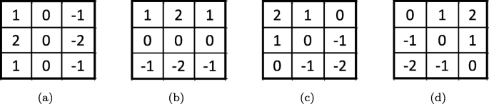

  

  The sobel mask for four kinds of direction a is horizontal mask (mx); b is vertical mask (my); c is 45^∘ mask (mxy); d is 135^∘ mask (myx)

  We use Eqs. (11)–(14) to calculate the gradient information of the vertical direction Δx, the gradient information of the horizontal direction Δy, the gradient information of the 45^∘ direction Δxy, and the gradient information of the 135^∘ direction Δyx.

  $$ \Delta x = |mx\times {\text{MPI}}| $$

  (11)
  $$ \Delta y = |my\times {\text{MPI}}| $$

  (12)
  $$ \Delta xy = |mxy\times {\text{MPI}}| $$

  (13)
  $$ \Delta yx = |myx\times {\text{MPI}}| $$

  (14)

• 5. In order to generate the estimated image EI, we calculate the missing image MI by four kinds of gradient information Δx, Δy, Δxy, and Δyx, as indicated in Eqs. (15)–(22). With Eqs. (15)–(22), we can generate eight weights of the eight neighboring positions, x_weight1, x_weight2, y_weight1, y_weight2, xy_weight1, xy_weight2, yx_weight1, and yx_weight2, as shown in Fig. 5.

  $$ \begin{aligned} x\_\text{weight1}&=\text{Weight}/\left(\Delta x(i,j)+{\text{Coe}}\times \Delta x(i,j-1)\right.\\ &\quad\left.+\Delta x(i,j-2)+1\right) \end{aligned} $$

  (15)

  Fig. 5

  

  The positions of the eight weights

  $$ \begin{aligned} x\_\text{weight2}&=\text{Weight}/\left(\Delta x(i,j)+{\text{Coe}}\times \Delta x(i,j+1)\right.\\ &\quad\left.+\Delta x(i,j+2)+1\right) \end{aligned} $$

  (16)
  $$ \begin{aligned} y\_\text{weight1}&=\text{Weight}/\left(\Delta y(i,j)+{\text{Coe}}\times \Delta y(i-1,j)\right.\\ &\quad\left.+\Delta y(i-2,j)+1\right) \end{aligned} $$

  (17)
  $$ \begin{aligned} y\_\text{weight2}&=\text{Weight}/\left(\Delta y(i,j)+{\text{Coe}}\times \Delta y(i+1,j)\right.\\ &\quad\left.+\Delta y(i+2,j)+1\right) \end{aligned} $$

  (18)
  $$ {}\begin{aligned} xy\_\text{weight1}&=\text{Weight}/\left(\Delta xy(i,j)+{\text{Coe}}\!\times\! \Delta xy(i\,-\,1,j\,-\,1)\right.\\ &\quad\left.+\Delta xy(i-2,j-2)+1\right) \end{aligned} $$

  (19)
  $$ {}\begin{aligned} xy\_\text{weight2}&\,=\,\text{Weight}/\!\left(\!\Delta xy(i,j)+{\text{Coe}}\times \Delta xy(i+1,j+1)\right.\\ &\quad\left.+\Delta xy(i+2,j+2)+1\right) \end{aligned} $$

  (20)
  $$ {}\begin{aligned} yx\_\text{weight1}&\,=\,\text{Weight}/\left(\Delta yx(i,j)+{\text{Coe}}\times \Delta yx(i\,-\,1,j+1)\right.\\ &\left.+\Delta y(i-2,j+2)+1\right) \end{aligned} $$

  (21)
  $$ {}\begin{aligned} yx\_\text{weight2}&\,=\,\text{Weight}/\!\left(\!\Delta yx(i,j)\,+\,{\text{Coe}}\!\times\! \Delta yx(i+1,j-1)\right.\\ &\left.+\Delta y(i+2,j-2)+1\right) \end{aligned} $$

  (22)

  Where Weight and Coe are two weight parameters. In general, the closer the positions are, the more information is provided, such as the vertical weight and the horizontal weight. In contrast, the farther position results in the lack of the information provided, such as the 45^∘ weight and 135^∘ weight. Therefore, we use two parameters Weight and Coe to adjust the weight of the rule. In this paper, we apply PSO algorithm [30] to estimate the most appropriate weight values. This algorithm is applied to solve optimization problems, and refer to Section 4.3. On the other hand, if the amount of gradient information of the neighboring pixel is tremendous, the neighboring pixel contributes less to predict the central pixel. On the contrary, the pixel has more contribution. Moreover, the eight weights of the eight neighboring pixels are utilized by Eq. (23) to estimate the 5×5 estimated image P, where MI(i,j) represents one pixel of the missing image MI.

  $$ {}\begin{aligned} P(i,j)&=\left\lfloor \left(x\_{\text{weight}}1\times {\text{MI}}(i,j-1)+x\_{\text{weight}}2\times {\text{MI}}(i,j+1)\right.\right. \\ &+y\_{{\text{weight}}1}\times {\text{MI}}(i-1,j)+y\_{{\text{weight}}2}\times {\text{MI}}(i+1,j) \\ &+xy\_{{\text{weight}}1}\times {\text{MI}}(i-1,j-1)\,+\,xy\_{{\text{weight}}2}\times {\text{MI}}(i+\!1,j\,+\,1) \\ &\left.+yx\_{{\text{weight}}1}\times {\text{MI}}(i-1,j+1)+y\_{{\text{weight}}2}\times {\text{MI}}(i+1,j\,-\,1)\right)\\ &\left./ {\text{weight}}\_{{\text{sum}}}\right\rfloor \\ {\text{where}} \\ {\text{weight}}\_{{\text{sum}}} &= x\_{{\text{weight}}1} + x\_{{\text{weight}}2} + y\_{{\text{weight}}1} + y\_{{\text{weight}}2} \\ &+ xy\_{{\text{weight}}1} + xy\_{{\text{weight}}2} + yx\_{{\text{weight}}1} + yx\_{{\text{weight}}2} \end{aligned} $$

  (23)

  Then, the 5×5 difference histogram e is generated from the difference values between the original image I and the estimated image P by Eq. (24).

  $$ e(i,j)=I(i,j)-P(i,j) $$

  (24)

3.2 Embedding algorithm

Assume T1 and T2 are two thresholds, where T1≥0 and T2<0. Before embedding, the T1 and T2 thresholds are decided appropriately by Section 3.4. Next, the embedding position are differentiated into allowing embedding or non-allowing embedding one by Section 3.3. If the position is allowing embedding, the message is embedded by Eq. (26). If the position is non-allowing embedding, the position is skipped. A key pseudo-random binary sequence generated by the encryption key is utilized to encrypt secret message w through exclusive-or operation, encryption data is generated h, as shown in Eq. (25).

$$ h=w \oplus {\text{key}} $$

(25)

The procedure of embedding message is described below:

$$ {}e'(i,j)= \left\{\begin{array}{ccc} e(i,j)+T1+1 & if & e(i,j)>T1\ {\text{and}}\ T1\geq0 \\ e(i,j)+T2 & if & e(i,j)<T2\ {\text{and}}\ T2<0 \\ 2e(i,j)+h & if & T2\leq e(i,j)\leq T1 \end{array}\right. $$

(26)

where h∈{0,1} is the current encrypted hidden bit.

After embedding the hidden data, the stego-image S is obtained as

$$ S(i,j)=e'(i,j)+P(i,j) $$

(27)

Likewise, embed the three sets cross, star, and circle as above. Finally, the stego-image S and two threshold values, T1 and T2 are outputted.

3.3 Embedding selection by non-linear regression analysis and self-block standard deviation statistics

By Section 3.2, we can know that the difference histogram e and two thresholds T1, T2 are utilized to embed messages. In general, the difference histogram is concentrated on 0, thus the 0 position is embedded preferentially when embedding. Next, move current position to the left or right for embedding, as shown in Section 3.4. When embedding messages, not all positions can be embedded, but in order to comply with the rule of a reversible data hiding method, all positions must be shifted, which leads to the reduction of image quality after embedding. Therefore, we hope design a rule that can classify these positions into allowing embedding positions and non-allowing embedding positions, and then reduce the unnecessary shifting to improve the image quality after embedding.

3.3.1 Training stage

First, we choose 30 nature images. Each image is passed through stage 1 to 4 of Section 3.1 to generate mirroring prediction image MPI and to calculate the standard deviation value of the current position σ_i,j by Eq. (28)

$$\begin{array}{@{}rcl@{}} \begin{aligned} \sigma_{i,j}&=\left|\sqrt{\frac{1}{8}\sum_{(i,j)\in\omega}[{\text{MPI}}_{i,j}-\overline{{\text{MPI}}}_{i,j}]^{2}} \right| \\ {\text{where}} \\ \overline{{\text{MPI}}}_{i,j}&=\frac{1}{8}\sum_{(i,j)\in\omega}{\text{MPI}}_{i,j} \\ \omega &= \left\{(i-1,j-1), (i+1,j+1), (i-1,j+1),(i+1,j-1), \right.\\ & \left.(i-1,j), (i+1,j), (i,j-1), (i,j+1)\right\} \end{aligned} \end{array} $$

(28)

Next, calculate the difference histogram e by the stage 5 of Section 3.1. The two thresholds T1=4, T2=− 4 are chosen to calculate the probability of the current position that difference histogram e(i,j) is T2≤e(i,j)≤T1 when standard deviation value is σ, and that is the probability of embedding EP(σ), as shown in Eq. (29)

$$\begin{array}{@{}rcl@{}} {\text{EP}}(\sigma) &=& \frac{{\text{EC}}(\sigma)}{{\text{EC}}(\sigma)+{\text{NEC}}(\sigma)} \\ {\text{where}}\ 0\leq \sigma \leq 49 \end{array} $$

(29)

Where EC is the embedding capacity, and NEC is the non-embedding capacity. Figure 6 indicates the histogram of the embedding probability, where x axis is the size of the standard deviation value σ, and y axis is the size of the embedding probability EP. We can find that when the lower the standard deviation leads to the higher probability of embedding, it represents the position is in a smooth region, thus it is easy to predict. Otherwise, this position is in a complex area, so it is difficult to predict. We set a threshold th, when σ(i,j)≤th, the position is used to embedding the message h by Eq. (26), otherwise, the position is skipped. During embedding, the embedding rage T1=4 and T2=− 4 are applied. We also utilize the 30 nature images to do the embedded statistics, where threshold th is 2, 4, 6, 8, 12, 16, 20, and 24. When the threshold th is the same and embedding rage T1=0∼4, T2=0∼− 4, we count the relation between the PSNR and the embedding capacity, as shown in Fig. 7, where the label origination denotes the threshold is not applied when embedding. Figure 7 shows that the best embedding threshold is different in different embedding capacity. It also shows that the image quality is really improved after embedding when the embedding threshold is used. We use non-linear regression analysis method to predict a quadratic curve function in each embedding threshold th, as shown in Eq. (30), where threshold th = 2,4,6,8,12,16,20,and24 and x is the embedding capacity.

$$ y({\text{th}},x)=a_{{\text{th}}}+b_{{\text{th}}}x+c_{{\text{th}}}x^{2} $$

(30)

Fig. 6

Histogram of the embedding probability

Fig. 7

The PSNR versus the capacity curves of using the different thresholds

Figure 8 shows the relation figure of the embedding capacity and the quality of the image when the threshold th = 12. The solid line is the line graph after statistics actually and the dotted line is the quadratic curve graph by using the non-linear regression analysis. Therefore, we can generate eight quadratic curve functions.

Fig. 8

The PSNR versus the capacity curves of using the 12 threshold and prediction function

3.3.2 Testing stage

Before embedding, if this image is the type that has many edges, the amount of the small standard deviation values is relatively small, such as standard deviation values = 1, 2, and 3. It would cause some problems like the amount of the embedding is limited or the embedding range is increased too much, which reduces the quality of the embedding. In order to avoid this special case, after generating mirroring prediction image MPI, count the amount of the current standard deviation value σ_i,j in advance, and then set the largest standard deviation value as initial value init_th.

Next, employ the capacity of the embedding message x to find the best threshold best_th by Eq. (31).

$$ {\text{best\_{th}}}=\arg\max_{{\text{th}}} y({\text{th}},x) $$

(31)

If best_th<init_th, the best threshold best_th=init_th. If the best threshold best_th≥init_th, the best_th is not changed. Finally, we can utilize the best threshold best_th to generate the best decision and to differentiate between embedding region and non-embedding region, and then needless shifting is reduced.

3.4 Automatic embedding range decision

In Sections 3.1 and 3.3, our method needs to decide the embedding rage T1 and T2. Therefore, we propose a method that can utilize the size of the embedding messages to generate the best range T1 and T2 automatically to achieve the best quality of the embedding, as show in Figs. 9 and 10.

Fig. 9

The flow diagram of generating initial embedding range

Fig. 10

The flow diagram of generating the best embedding range

The proposed methodology is described in two stages:

• 1. Generating an initial embedding range

  First, input the embedding messages x and the best_th be generated by Section 3.3. Next, initialize F_T1=0, F_T2=0 and D=R, and then employ F_T1, F_T2 and th to embed messages by the embedding method of Section 3.2. The embedding range is F_T1 and F_T2, while the amount that can be embedded is less than the capacity of embedded messages x, the embedding range expands to the left or right. In contrast, while the amount can be embedded is more than or equal to the capacity of embedded messages x, F_T1, F_T2, and D are outputted, where D is used to judge left or right for expansion. The aim is, when increasing the range, it would balance expand to the left or right from center to achieve the best image quality, as shown in Fig. 9.

• 2. Generating the best embedding range

  First, input the F_T1, F_T2 and D that be generated from stage 1 and the best_th that be generated from Section 3.3. We use the best_th to let the embedding position differentiate between allowing embedding and non-allowing embedding. Next, it is expanded to the left or right from center balanced again to generate another embedding range S_T1 and S_T2. We compare the image quality of the embedding range F_T1, F_T2 with the image quality of the embedding range S_T1, S_T2. Sometimes, it would add the total amount of the small standard deviation values by increasing the embedding range. This will increase the success rate of judging the embedded position and the non-embedded position, thereby increases the image quality after embedding. However, due to this condition, the condition would probably increase the unnecessary shifting to reduce the image quality after embedding. Therefore, we compare the image quality after embedding these two kinds of status and find the best method to output embedding range, as shown in Fig. 10.

Figure 11 shows the example of embedding hiding messages into a difference image. Assume x is 20,000 bits, and we get the results of 8 quadratic curve functions by Eq. (31), as follows:

• 1. th2:y=53.5,th4:y=55.3,th6:y=53.8,th8:y=53,

  Fig. 11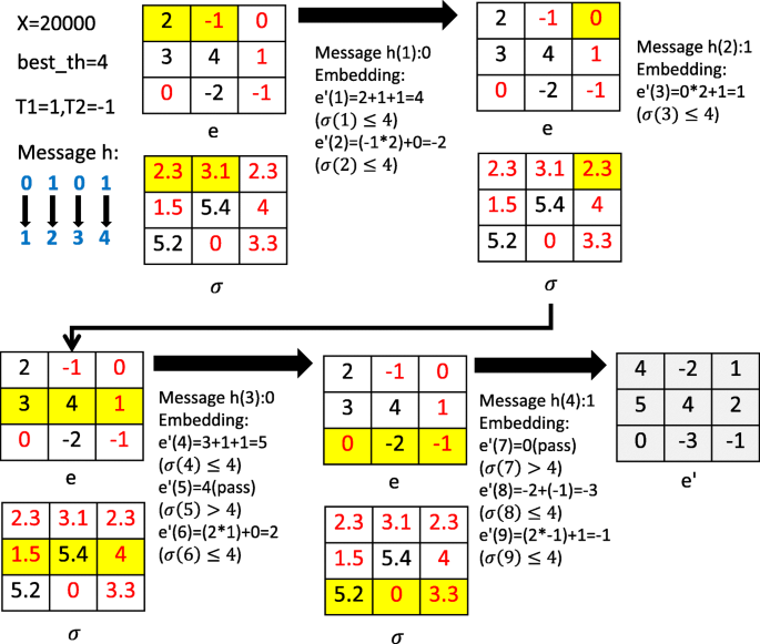

  

  Example of hiding data into an image of 3 x 3 pixels

• 2. th12:y=52.2,th16:y=51.8,th20:53.6,th24:y=53.4

among them the max y is th4, so best_th = 4.

If the embedding position’s standard deviation value σ≤ 4, the position is allowing embedding position, otherwise it is non-allowing embedding position. Assume a message h=0101. σ(1)≤ 4, this position is allowing embedding position. We can find that the position can be an embedded message when − 1≤e≤1 by Eq. (26); otherwise, it cannot be an embedded message, but it still needs to be shifted. Thus, e(1) = 2 cannot be an embedded message, but we still shift it. We can calculate e^′(1) = 4 by Eq. (26). Since σ(2)≤4, it is an allowing embedding position. e(2) = − 1 means it can be embedded message h(1) = 0, then we can calculate e^′(2) = − 2 by Eq. (26). Similarly, σ(3)≤4 is an allowing embedding position, e(3)=0 can be embedded message h(2) = 1, then e^′(3) = 1. σ(4) is an allowing embedded position, the position of e(4) cannot be an embedding message, thus e^′(4) = 5. σ(5) > 4, so it is a non-allowing embedding position, then e’(5) = 4 and it needs no shifting. e^′(6) = 2 is an allowing embedding position; it can be an embedded message h(3) = 0, then e^′(6) = 2. σ(7) is a non-allowing embedding position, then e^′(7) = 0 and it needs no shifting. σ(8) and σ(9) are allowing embedding positions, the position of e(8) cannot be an embedded message, then e^′(8) = − 3. The position of e(9) can be an embedded message h(4) = 1, then e^′(9) = − 1. Finally, the embedded difference image e^′ is generated.

3.5 Extracting and reversing algorithm

The procedure of message extraction and recovery are described below:

• 1. Divide 5×5 stego-image S into 4 groups: square, cross, star, and circle. We define the 4 groups as G1, G2, G3, G4, respectively. We only discuss G4 in this sub-section because G3, G2, G1 are the same cases.

• 2. Mirror the stego-image S into a 7×7 mirror image MS.

• 3. Hidden the G4 as missing image, and the four neighboring pixels are utilized to predict center pixel, and then a 5×5 prediction image PS is generated.

• 4. Mirror prediction image PS into a 9×9 mirror prediction image MPS.

• 5. Calculate the weights of the eight neighboring pixels. Then a 5×5 stego-estimated image P^′ is generated.

• 6. A 5×5 difference histogram e^′ is generated by Eq. (32).

  $$ e'(i,j)=S(i,j)-P'(i,j) $$

  (32)

• 7. The embedding position differentiates between allowing embedding and non-allowing embedding by Section 3.3. If the position is allowing embedding, the hiding bit h is extracted by Eq. (33). If the position is non-allowing embedding, the position is skipped.

  $$ h=e'(i,j)\ {\text{mod}}\ 2 \qquad if \quad 2\times T2 \leq e'(i,j) \leq 2\times T1 + 1 $$

  (33)

• 8. The key pseudo-random binary sequence is utilized to decrypt h through exclusive-or operation to get original secret message w.

• 9. If the position is allowing embedding, original error prediction e(i,j) is obtained by Eq. (34). If the position is non-allowing embedding, e(i,j)=e^′(i,j).

  $$ {}e(i,j)\,=\, \left\{\!\!\begin{array}{ccc} e'(i,j)-T1-1 & {\text{if}} & e'(i,j)>2\times T1+1 \\ e'(i,j)-T2 & {\text{if}} & e'(i,j)<2\times T2 \\ \lfloor e'(i,j)/2 \rfloor & {\text{if}} & 2\times T2 \leq e'(i,j) \leq 2\!\times\! T1 + 1 \end{array}\right. $$

  (34)

  Recovery of the value of the original image I(i,j) is as follows:

  $$ I(i,j)=e(i,j)+P(i,j) $$

  (35)

Figure 12 shows the example of message extraction and recovery image. Assume x is 20,000 bits, the best_th = 4 can be calculated by Eq. (34), and T1=1, T2 = − 1. σ(1) and σ(2) are less than or equal to best_th, e^′(1) and e^′(2) are allowing embedding positions. We can find that − 2≤e^′≤3 is a position of the embedded message by Eq. (34). Otherwise, it is a position of the non-embedded message. Therefore, e^′(1) = 4, the position is a position of the non-embedded message, then we can calculate e(1) = 2 by Eq. (34). e^′(2) = − 2 is a position of the embedded message, it can be calculated h^′(1) = 0 by Eq. (33) and it can be recovered e(2) = − 1 by Eq. (34). Similarly, e^′(3) is an allowing embedding position, and it is also a position of the embedded message, then h^′(2) = 1, e(3) = 0. σ(4) is an allowing embedding position, and e^′(4) is a position of the non-embedded message, then e(4) = 3. σ(5) > 4 is a non-allowing embedding position, then e(5) = 4, it need not shifting. σ(6) is a allowing embedding position, e^′(6) is a position of the embedded message, then h^′(3) = 0, e(6) = 1. σ(7) is a non-allowing embedding position, then e(7) = 0, it needs no shifting. σ(8) and σ(9) are allowing embedding positions, e^′(8) is a position of the non-embedded message, e(8) = − 2. e^′(9) is a position of the embedded message, then h^′(4)=1, e(9) = − 1. Finally, the message h^′=0101 and the reduced difference image e can be generated.

Fig. 12

Example of extraction and recovery from a processed image of 3 x 3 pixels

3.6 Overflow and underflow problem

A stego-image S is generated from Section 3.2. If the pixel is outside of 0∼255, it is called overflow or underflow. It cannot recover after embedding. Therefore, in embedding stage, we must consider this problem. This study uses the solution proposed by [13]. It is described below:

• 1. Construct the m×n location map L, where m, n is the length and width of the original image I, respectively. Then, set all the positions L(i)=1.

• 2. If embedding positions e(i,j) is [1,254], set L(i)=0 and embedding message. Otherwise, set L(i)=1 and switch into the next embeddable position.

• 3. Encode the location map L by the lossless compression.

• 4. Record the least significant bits of first 2⌈log₂(m×n)⌉+LS image pixels where LS is the length of the compressed location map L.

During decoding processing, first the compressed location map L is reconstructed from 2⌈log₂(m×n)⌉+LS image pixels of marked image. Then, the original location map is further generated by lossless decompression. Finally, the secret message is extracted and the host image is recovered.

4 Experimental results and discussions

In this section, the proposed method was compared with five methods, Kim et al. (2009) [9], Sachnev et al. (2009) [12], Luo et al. (2011) [10], Zhao et al.(2011) [11],and Rad et al. (2016) [13]. In the experiments, all standard 512×512 grayscale images were served as test images, including Baboon, Lena, Peppers, Elaine, Boat, and Barbara from the USC-SIPI standard testing database [29] and 1000 natural images that we collected. The proposed method was implemented using MATLAB Version R2012a on Intel Core i5 2.5 MHz with 8 G of memory. In the prediction stage, after deciding the embedding range, the two parameters Weight and Coe were used, as shown in Table 1. In the embedding selection stage, the non-linear regression analysis was applied to estimate eight quadratic curve functions; these functions are as follows:

$$\begin{aligned} {\text{th}}= 2:\quad y = -~7E-09x^{2} - 0.0005x + 66.399 \\ {\text{th}}= 4:\quad y = -~2E-10x^{2} - 0.0002x + 59.458 \\ {\text{th}}= 6:\quad y = 3E-10x^{2} - 0.0002x + 57.761 \\ {\text{th}}= 8:\quad y = 3E-10x^{2} - 0.0002x + 56.96 \\ {\text{th}}=12:\quad y = 3E-10x^{2} - 0.0002x + 56.171 \\ {\text{th}}=16:\quad y = 3E-10x^{2} - 0.0002x + 55.771 \\ {\text{th}}=20:\quad y = 3E-10x^{2} - 0.0001x + 55.511 \\ {\text{th}}=24:\quad y = 2E-10x^{2} - 0.0001x + 55.326 \end{aligned} $$

Table 1 Optimum results in different thresholds

4.1 Prediction difference histograms comparison

In this sub-section, the proposed prediction method was compared with five methods. It can be found that the difference histograms that we proposed the prediction method in Boat image and Peppers image are more concentrated and the peaks are higher than other methods. The prediction performance is better especially in a smooth image, as shown in Fig. 13. In general, the more concentrated the different histogram is and the higher the peak is, the more accurate the prediction result is. Therefore, our method can reduce the probability of needless shifting to get huge embedding capacity and good embedding quality.

Fig. 13

The prediction error histograms. a Boat image. b Peppers image

4.2 Comparison hiding rate versus image quality

In this sub-section, the embedding capacity and image quality of proposed embedding method was compared with other five methods. In general, peak signal-to-noise ratio (PSNR) and structural similarity (SSIM) for embedding capacity are two kinds of performance indicators. The bigger the value of PSNR, the smaller the image distortion rate, where PSNR is defined as Eq. (36).

$$ {}{({\text{dB}}})~=~10\log_{10}\frac{255^{2}}{\frac{1}{m\times n}\sum_{x~=~0}^{m-1}\sum_{y~=~0}^{n-1}\bigl[X(x,y)-X'(x,y)\bigr]} $$

(36)

Where X(i,j) is an original image, and X^′ is a cover image.

The SSIM index is calculated on various windows of an image. The measure between two images x and y of common size m×n is:

$$ {\text{SSIM}}(x,y)=\frac{(2\mu_{x}\mu_{y}+c_{1})(2\sigma_{xy}+c_{2})} {(\mu_{x}^{2}+\mu_{y}^{2}+c_{1})(\sigma_{x}^{2}+\sigma_{y}^{2}+c_{2})} $$

(37)

Where x is an original image, and y is a cover image, μ_x is the average of x, μ_y is the average of y, $\sigma _{x}^{2}$ is the variance of x, $\sigma _{y}^{2}$ is the variance of y, σ_xy is the covariance of x and y, c1=(k1L)² and c2=(k2L)² are two variables to stabilize the division with weak denominator, L is the dynamic range of the pixel-values, k1 = 0.01 and k2 =0.03 small constants near zero [31]. The value of SSIM index belongs to [0,1]. When the two images are identical, the value of the SSIM similarity is 1. The capacity of cover image is defined as Eq. (38).

$$ {\text{Capacity}}=\frac{{\text{hidden}}\_{\text{bits}}}{m\times n} $$

(38)

Where hidden_bits is the total number of hidden bits, and m and n represent the length and width, respectively.

In our experiments, it is verified that the hidden message can be extracted and the original image can be reconstructed by our method. We used six test image to draw the curve graph of the PSNR and the embedding capacity, as shown in Fig. 14. It can be found that at the same capacity, our proposed RDH algorithm achieve the best image quality among the six RDH algorithms. Therefore, it can demonstrate the embedding performance can be improved with our method. In our experiments, it is verified that the hidden message can be extracted and the original image can be reconstructed by our method. Figure 14 shows the PSNR and the embedding capacity that generated by five RDH algorithms and our method for the test images: Baboon, Lena, Peppers, Elaine, Boat, and Barbara.

Fig. 14

The PSNR versus the capacity curves of the seven compared RDH algorithms for the test images. a Baboon. b Lena. c Peppers. d Elaine. e Boat. f Barbara

In addition, we make the statistic of the embedding capacity and PSNR and SSIM with 1000 natural images that we collected, and then the embedding capacity, PSNR and SSIM are averaged to draw a curve graph, as shown in Fig. 15. It can be found that our proposed method can more improve the embedding capacity and embedding quality more than the others.

Fig. 15

The PSNR and SSIM versus the capacity curves of the six compared RDH algorithms for the 1000 images. a PSNR. b SSIM

4.3 Parameter estimation

In this study, the two parameters Weight and Coe were utilized in prediction stage, referring to Section 3.1. We utilized 30 nature images and measured the optimal parameters of T1 and T2 at different embedding threshold values through an optimal algorithm, particle swarm optimization (PSO) [30]. A definition of the objective function of the optimal algorithm is provided in Eq. (39).

$$ \max\sum_{{\text{Image}}~=~1}^{30}{\text{Capacity(Image)}} $$

(39)

Where Image is a training image. The result of the optimal parameters we obtained was given in Table 1. Figure 16a shows the plot of the relation between generation number and fitness value, where the horizontal axis is the number of generation number and the vertical axis is the fitness value. Figure 16b shows the plot of generation number and coefficient value, where the horizontal axis is the number of generation number, the vertical axis is the coefficient value, W is the coefficient Weight and C is the coefficient Coe.

Fig. 16

Generation number comparison (a) vs. fitness value; (b) vs. coefficient value

4.4 Performance comparison of the four neighborhood and eight neighborhood with our method

Before the prediction stage, all pixels of this image are classified. Therefore, we compare the four neighboring pixels with the eight neighboring pixels at the same conditioning embedding stage. First, we divide all pixels of the image into two groups and utilized the four neighboring pixels to calculate and predict. Then, all pixels of the image are divided into four groups, and we employed the eight neighboring pixels to calculate and predict. We make the statistics of the embedding capacity and PSNR with six test images, including Baboon, Lena, Peppers, Elaine, Boat, and Barbara, and then the embedding capacity and PSNR are averaged to draw a curve graph, as shown in Fig. 17. It can be found that using the eight neighboring pixels can more improve the embedding capacity and embedding quality by than the four neighboring pixels.

Fig. 17

Performance comparison of the four neighborhood and eight neighborhood with our method

4.5 Comparison of embedding after sorting and selection embedding

In our embedding stage, the best standard deviation value threshold will be generated to achieve optimal embedding performance. Therefore, we compare below two embedding methods. One is the embedding after sorting; it is embedded after sorting by the size of the standard deviation values. The other is the selection embedding; it first makes to sort by the size of the standard deviation value, next if the value of the current position is less than the standard deviation value threshold, and the position will be embedded messages; otherwise, there will be no change. We make the statistics of the embedding capacity and PSNR with six test images, including Baboon, Lena, Peppers, Elaine, Boat, and Barbara, and then the embedding capacity and PSNR to draw a curve graph, as shown in Fig. 18. It can be found using the selection embedding method can improve the embedding capacity and the embedding quality of this system, in particular, when the embedding capacity is small. We also compare with three test images, including Baboon, Lena, and Peppers, as shown in Tables 2, 3, and 4, where label Proposed is embedding from left to right, from top to bottom. Label Proposed(sort) is embedded after sorting with standard deviation value. Label Proposed (selection) is sorted by the size of the standard deviation value. Next, if the value of the current position is smaller than the standard deviation value threshold, we embed messages in the current position; otherwise, there will be no change. We find that sorting with standard deviation value in the same embedding condition improve the embedding capacity. If we further process images by selection embedding, we can further improve the embedding capacity. Besides, the performance is better for complex images than smooth images, in particular, when the embedding capacity is small.

Fig. 18

Performance comparison of the original method and embedding selection method

Table 2 Comparison of PSNR and SSIM for our schemes on Baboon image

Table 3 Comparison of PSNR and SSIM for our schemes on Lena image

Table 4 Comparison of PSNR and SSIM for our schemes on Boat image

4.6 Comparison of automatic embedding range decision

In our system, we can find the best embedding range by the size of the embedding capacity for the user. We used four test images, Baboon, Lena, Boat, and Peppers, and the embedding capacities are 10,000 and 20,000, respectively, as shown in Table 5 and 6, where selection 1 is the quality of PSNR generated in stage one, and selection 2 is the quality of PSNR generated in stage two. It can be found that the embedding range can be expanded once to obtain better image quality when the amount of embedding is small. However, the expansion of embedding range is not absolutely better when the amount of embedding is large. Therefore, it compares the image qualities of two embedding ranges in the second stage, and then it would generate the optimal embedding range.

Table 5 Comparison of [PSNR,SSIM] for two stages (messages = 10,000)

Table 6 Comparison of [PSNR,SSIM] for two stages (messages = 20,000)

4.7 Comparison of the executing-time performance

The execution-time performance comparison among the concerned six RHD algorithms, as shown in Table 7. We can find that method Kim et al. (2009) proposed has the best execution-time performance, because it only used a simple shifting. Rad et al. (2016) proposed method has the worst execution-time performing, because the embedded rule processing is applied. Then, our proposed methods, Label Proposed, needs a little bit more embedding time due to the following two main factors. One, the original image is divided into four groups. Second, multi-directional gradient prediction is calculated. Label Proposed (sort) needs more time, because it is embedding after sorting with standard deviation value. Finally, Label Proposed (select) is determining whether the position is suitable for embedding messages. If it is not suitable, it needs to determine the next position, so it also affects a little processing time.

Table 7 The execution-time comparison among the concerned five RHD algorithms and our methods

5 Conclusions

In this paper, we proposed a new multi-directional gradient prediction method to generate more accurate prediction result. Next, in embedding stage, according to the embedding capacity of information, we generate the best decision based on non-linear regression analysis, which can differentiate between embedding region and non-embedding region, and then needless shifting was reduced. Finally, we employ automatic embedding range decision with sorting by the amount of regional variance. It can be prioritized to embed for the region which was easy to predict, and the quality of the image was improved after embedding. The experimental results showed our difference histograms of the proposed prediction method are more concentrated and their peak are higher than other methods. In the selection of embedding method, experimental results indicated our method can improve embedding performance, especially when the image is a complex or the amount of embedding is small. Moreover, the experimental results also demonstrated that the embedding capacity of our proposed the method outperforms other methods with less distortion. In the future, we hope to apply the proposed method to JPEG reversible data hiding and encrypted image reversible data hiding.

References

J. Fridrich, M. Goljan, R. Du, in SPIE 2001. Invertible authentication (International Society for Optics and Photonics, SPIE, 2001), pp. 197–208. https://doi.org/10.1109/itcc.2001.918795.
J. Fridrich, M. Goljan, R. Du, Lossless data embedding-newparadigm in digital watermarking. EURASIP J. Appl. Signal Process.2:, 185–196 (2002).
M. U. Celik, G. Sharma, A. M. Tekalp, E. Saber, Lossless generalized-lsb data embedding. IEEE Trans. Image Process.14(2), 253–266 (2005). https://doi.org/10.1109/tip.2004.840686.
M. U. Celik, G. Sharma, A. M. Tekalp, Lossless watermarking for image authentication: A new framework and an implementation. IEEE Trans. Image Process.15(4), 1042–1049 (2006). https://doi.org/10.1109/tip.2005.863053.
J. Tian, Reversible data embedding using a difference expansion. IEEE Trans. Circuits Syst. Video Technol.13:, 890–896 (2003).
M. Alattar, in Int. Conf. Image Process. Reversible watermark using difference expansion of triplets (IEEE, 2003), pp. 501–504. https://doi.org/10.1109/icip.2003.1247008.
M. Alattar, in Int. Conf. Image Process. Reversible watermark using difference expansion of quads (IEEE, 2004), pp. 377–380. https://doi.org/10.1109/icassp.2004.1326560.
Z. Ni, Y. Q. Shi, N. Ansari, W. Su, Reversible data hiding. IEEE Trans. Circuits Syst. Video Technol.16:, 354–362 (2006).
K. S. Kim, M. J. Lee, H. Y. Lee, H. K. Lee, Reversible data hiding exploiting spatial correlation between sub-sampled images. Pattern Recog.42:, 3083–3096 (2009).
H. Luo, F. X. Yu, H. Chen, Z. L. Huang, P. H. Wang, Reversible data hiding based on block median preservation. J. Inf. Sci.181:, 308–328 (2011).
Z. Zhao, H. Luo, Z. M. Lu, J. S. Pan, Reversible data hiding based on multilevel histogram modification and sequential recovery. Int. J. Electron. Commun.65:, 814–826 (2011).
V. Sachnev, H. J. Kim, J. Nam, S. Suresh, Y. Q. Shi, Reversible watermarking algorithm using sorting and prediction. IEEE Trans. Circ. Syst. Video Technol.19:, 989–999 (2009).
R. M. Rad, K. Wong, J. M. Guo, Reversible data hiding by adaptive group modification on histogram of prediction errors. Signal Process.125:, 315–328 (2016).
R. M. Rad, K. Wong, J. M. Guo, A unified data embedding and scrambling method. IEEE Trans. Image Process.23:, 1463–1475 (2014).
C. Qin, C. C. Chang, Y. H. Huang, L. T. Liao, An inpainting-assisted reversible steganographic scheme using a histogram shifting mechanism. IEEE Trans. Circ. Syst. Video Technol.7:, 1109–1118 (2013).
X. Li, L. B., B. Yang, T. Zeng, General framework to histogram-shifting-based reversible data hiding. IEEE Trans. Image Process.6:, 2181–2191 (2013).
H. J. Hwang, S. H. Kim, H. J. Kim, Reversible data hiding using least square predictor via the lasso. EURASIP J. Image Video Process.42:, 1–12 (2016).
J. N. J. Wang, X. Zhang, Y. Q. Shi, Rate and distortion optimization for reversible data hiding using multiple histogram shifting. IEEE Trans. Cybernet.47:, 315–326 (2017).
F. Huang, K. X. Qu, J. Huang, Reversible data hiding in jpeg images. IEEE Trans. Circ. Syst. Video Technol.26:, 1610–1621 (2016).
D. Hou, H. Wang, W. Zhang, Reversible data hiding in jpeg image based on dct frequency and block selection. Signal Process.148:, 41–47 (2018).
X. C. Cao, X. X. Wei, D. Meng, X. J. Guo, High capacity reversible data hiding in encrypted images by patch-level sparse representation. IEEE Trans. Cybern.46:, 1132–1143 (2016).
K. D. Ma, X. F. Zhao, N. H. Yu, F. H. Li, Reversible data hiding in encrypted images by reserving room before encryption. IEEE Trans. Inf. Forensics Secur.8:, 553–562 (2013).
X. Zhang, Z. Qian, G. Feng, Y. Ren, Efficient reversible data hiding in encrypted images. J. Vis. Commun. Image Represent.25:, 322–328 (2014).
F. J. Huang, J. W. Huang, Y. Q. Shi, New framework for reversible data hiding in encrypted domain. IEEE Trans. Inf. Forensics Secur.11:, 2777–2789 (2016).
Z. X. Qian, X. P. Zhang, G. R. Feng, Reversible data hiding in encrypted images based on progressive recovery. IEEE Signal Process. Lett.23:, 1672–1676 (2016).
Z. X. Qian, X. P. Zhang, Y. L. Ren, G. R. Feng, Block cipher based on separable reversible data hiding in encrypted images. Multimedia Tools Appl.75:, 13749–13763 (2016).
C. Qin, Z. He, X. Luo, J. Dong, Reversible data hiding in encrypted image with separable capability and high embedding capacity. Inf. Sci.465:, 285–304 (2018).
C. Qin, W. Zhang, F. Cao, X. Zhang, C. C. Chang, Separable reversible data hiding in encrypted images via adaptive embedding strategy with block selection. Signal Process.153:, 109–122 (2018).
USC-SIPI Image Database. http://sipi.usc.edu/services/database/Database.html. Accessed Aug 2019.
J. Kennedy, R. Eberhart, in ICNN’95 - International Conference on Neural Networks. Particle swarm optimization (IEEE, 1995).
Z. Wang, A. C. Bovik, H. R. Sheikh, E. P. Simoncelli, Image quality assessment: from error visibility to structural similarity. IEEE Trans. Image Process.13:, 600–612 (2004).
Acknowledgements
We would like to thank several anonymous reviewers and the editor for their comments.
Funding
This research received no external funding.
Author information
Authors and Affiliations
Contributions
HKM invented the proposed idea. CHY participated in the statistical theory to back up and support the proposed idea. HKM, CHY2, and LMC helped in the investigation. CHY2 and LMC wrote the original draft. HKM, CHY1, CHY2, and LMC contributed to the writing, review, and editing of CHY1, CHY2 participated in the design and coordination of paper and finish manuscript of the paper. The authors read and approved the final manuscript.
Corresponding author
Ethics declarations
Competing interests
The authors declare that they have no competing interests.
Additional information
Publisher’s Note
Springer Nature remains neutral with regard to jurisdictional claims in published maps and institutional affiliations.
Rights and permissions
Open Access This article is distributed under the terms of the Creative Commons Attribution 4.0 International License(http://creativecommons.org/licenses/by/4.0/), which permits unrestricted use, distribution, and reproduction in any medium, provided you give appropriate credit to the original author(s) and the source, provide a link to the Creative Commons license, and indicate if changes were made.
About this article
Cite this article
Hung, KM., Yih, CH., Yeh, CH. et al. A high capacity reversible data hiding through multi-directional gradient prediction, non-linear regression analysis and embedding selection. J Image Video Proc. 2020, 8 (2020). https://doi.org/10.1186/s13640-020-0495-7
Received:
Accepted:
Published:
DOI: https://doi.org/10.1186/s13640-020-0495-7