Mice endplate segmentation from micro-CT data through graph-based trabecula recognition

Abstract

Though segmentation of spinal column from medical images have been intensively studied for decade, most of the works were concentrated on the segmentation of the vertebral body and arch, instead of the endplate. Recently, the increasing study on degeneration analysis of vertebra and intervertebral disc (IVD) make endplate segmentation as important as others. While the accurately segmentation of mice endplate from micro computed tomography (CT) images is challenging. The major difficulties include potential high system payload and poor run-time efficiency resulting from high-resolution micro-CT data, highly complicated and variable shape of the vertebra tissues, and the ambiguous segmentation boundary due to the similarity of spongy structures inside both the endplate and its adjacent vertebral body. To solve the problems, the core idea of the proposed method is to identify trabeculae between the endplate and the body through a graph-based strategy. In addition, in order to reduce the data complexity, an endplate-targeted region of interest (ROI) extraction method is introduced according to the analysis of spatial relationship and variety of bone density of vertebra. Furthermore, shape priori of endplate in both two-dimensional and three-dimensional are extracted to assist in the segmentation. Finally, an iterative cutting procedure is implemented to produce the final result. Experiments were carried out which validate the performances of the proposed method in terms of effectiveness and accuracy.

1 Introduction

Demanded by image-based spine assessment, biomechanical modeling and surgery simulation, segmentation of spinal column from medical images have been intensively studied for decades. In former researches, most of the works were concentrated on segmenting vertebral tissues such as the body and arch, while vertebral endplate segmentation were rarely mentioned. However, endplate is as important as the others. As a transitional zone between the intervertebral disc (IVD) and vertebra, it not only plays an important role in containing the adjacent disc, distributing applied loads evenly to the underlying vertebra, but also serves as a semi-permeable interface that allows the transfer of water and solutes, preventing the loss of large proteoglycan molecules from the disc [1, 2]. Recently, it is also believed that there has a close relationship between the harm of endplate and osteoporosis [3]. Therefore, endplate segmentation could become an important pre-requisite of vertebra/IVD degeneration analysis and many other applications, which is a major motivation of this work.

Up to now, endplate segmentation from computed tomography (CT) images accurately is still a challenging task in practice, which relies heavily on knowledge, experience, and manual works [4]. The main difficulties can be concluded as follows.

• Potential high system payload and poor run-time efficiency. The average thickness of endplate is generally less than 80 μm; therefore, a high-resolution imagery such as the micro-CT technique is required in order to achieve a high-accuracy segmentation. While, high resolution often leads to high system payload and poor run-time efficiency.

• Highly complicated and variable shape of the vertebra tissues. The shape of vertebra including the endplate, body and arch are highly complicated and variable. For example, the mice vertebra mice we test have transverse processes relatively longer and of larger curvature comparing to the human’s. Therefore, mice vertebral body and arch are more likely to be interrupted with each other; it is more difficult to separate them properly. Besides, existing algorithms designed for human vertebrae may not be suitable for our case anymore.

• Ambiguous segmentation boundary. Both the endplate and body are composed of spongy cancellous bone (see blue and green region marked in Fig. 1a), which makes the segmentation boundary ambiguous. Though there exists a gap area (labeled with a yellow dotted line in Fig. 1b) between them, however, the gap is considerably narrow and divided by trabeculae, which means it is difficult to find a proper continuous curve as a segmentation boundary.

  Fig. 1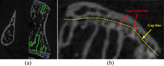

  

  Demonstration of endplate segmentation difficulties. a A sagittal view of the micro-CT data, where the blue and green marked the spongy structure caused by the cancellous bone. b Zoom in view of the endplate and its adjacent vertebral body region, where two of the gap trabecular and the gap line are labeled in red and yellow respectively

As we mentioned above, though few works could be found on endplate segmentation, plenty of researches have been done to achieve detection and segmentation of vertebrae [5–9], spinal canals [10], and spinal cord [11].

For the purpose of separating the neighboring vertebrae roughly, Zhao et al. [12] proposed a neighboring point rating method based on constructing membership grade to form a virtual plane to cut adjacent processes. The method proposed by Kim et al. [9] searches a ray emitted from the stared point among the center axis of the spine and further construct a three-dimensional (3D) surface by propagating the ray to detect the accurate gap area between two processes.

A common strategy to reduce the data complexity is by limiting the algorithm applied to a relatively small region of interest (ROI) [13]. In order to identify the ROI, Athertya et al. [5] extract the Harris corners [14] among the possible vertebra region to detect the vertebra range. However, the detection needs several interactions and training in advance, meanwhile the accuracy of detection depends on the selection of multi-stage seed points. Cheng et al. [6] detect the vertebra region by a probabilistic map computed from a voxel-wise classifier and use mean shift algorithm to estimate the ROI after annotations.

In our work, we also need to isolate individual vertebra from a given vertebral column, to extract the ROI for data complexity reduction, while more importantly, to segment the endplate, and we made it in a endplate-targeted way. Specifically, taking micro-CT images as input, we aim to develop an intelligent framework to accurately segment the endplate from the others. And the core idea is to recognize the trabeculae (e.g., marked by red circles in Fig. 1b) within the narrow gap formed by the endplate and its adjacent vertebral body by a graph-based algorithm. The proposed framework can be separated into four parts, which are (1) pre-processing, (2) priori shape extraction, (3) gap trabecula detection, and (4) trabecula cutting and refining. Particularly, we firstly isolate each vertebra and identify the ROI for endplate in a top-down basis (Section 2.1). Secondly, shape priori in both 2D and 3D are introduced to offer constraints for later graph cuts based trabeculae recognition (Section 2.2). After that, a graph will be constructed based on mask skeletonization before the graph cuts based trabeculae recognition (Section 2.3). Finally, we find an optimal cutting strategy to remove the redundant connections properly (Section 2.4). An accurate result can be achieved after these processes, which is ready for subsequent operations such as the 3D reconstruction.

2 Material and methods

The experimental data we used were collected from the animal laboratory of spinal surgery of the Xiangya Hospital. Micro-CT technique is adopted due to the high-quality imagery requirement. To capture the data, mice of different ages were fixed in a slot scanned by a Bruker SkyScan1172 micro-CT scanner. The in-plane resolution of the image is 7.27 μm × 7.27 μm, and the slice spacing is 7.27 μm. Figure 2 demonstrates a typical data of the inputs, which contains 4 lumbar vertebrae.

Fig. 2

The sagittal, coronal, and axial views of the input data

2.1 Pre-processing

The aim of the pre-processing is to get proper ROI for the endplates. In this work, a top-down strategy which consists of three steps as shown in Fig. 3 is proposed to achieve the goal from coarse to fine.

Fig. 3

The workflow of the proposed pre-processing

The first step is to isolate the vertebra from each others. Other than finding separation lines or surfaces such as the method proposed by Kim et al. [9], thanks to the high resolution of micro-CT image and unconnected spatial relationship among different vertebrae, this step can easily be done by 3D region growing on the mask resulting from a Otsu threshold.

The second step finds out ROI for endplate within each axial slices. Due to the shape complexity mentioned above, it is normally impossible to completely cut off the vertebral arch by planes as proposed in existed methods [12, 15]. To remove useless regions as many as possible, an optimal cylinder will be computed automatically in our method to meet the quasi-cylindrical shape of the vertebral body as shown in the right of Fig. 4. The cylinder can be obtained by topology analysis of the vertebra beginning from both the top and bottom part to the center part in axial planes slice by slice as indicated by blue arrows in Fig. 4. Because in this way, we could find two regions indicated by R₁ and R₂ in Fig. 4 which cover the entire endplate. Then, based on the projection of bone regions within R₁ and R₂, we can easily find a circle (e.g., C₁ in Fig. 4) which can be used to define the target cylinder.

Fig. 4

Vertebral arch removal

The last step produces the finest ROI by further confirming the proper range of the axial slices. It travels each slice in the way as described in the second step, while other than analyzing the topology, bone density ρ(I_i) of each slice i will be calculated according to Eq. 1, and then the variation of bone density will be used to find the rightful indexes.

$$\begin{array}{@{}rcl@{}} \rho(I_{i})=\frac{N_{F}(I_{i})}{A_{F}(I_{i})}\times 100\% \end{array} $$

(1)

where A_F(I_i) is the area (measured by number of pixels) of the entire vertebral region within slice I_i, while N_F(I_i) denotes the region where identified as the bone tissue within A_F(I_i) (e.g., the colored region of slice in Fig. 5a).

Fig. 5

Endplate region extraction. a Axial views (right) of four typical slices of index a, b, c, and d (left). b Bone density variation among a sequence of slices. The horizontal axis is the slice index, the vertical axis is the bone density value accordingly, P1 and P2 indicate the range of the result

The effect of this method lies in the fact that, as shown in Fig. 5a, the top layer of endplate is much denser than the other parts. For example, ρ(I_a)>ρ(I_b)>ρ(I_c)>ρ(I_d). With the computed data, a chart, as illustrated in Fig. 5b, can be used to find the desirable range. The horizontal axis of the chart is the slice index, the vertical axis is the bone density accordingly. For the case shown in Fig. 5b, P1 and P2 will be chosen as the bounds of the range. Because, along with the direction of the horizontal axis, ρ(I_P1) reaches the first peak and the variation of bone density around I_P2 become very small.

2.2 Shape priori extraction

It is well known that shape priori could be very useful because the constraints they represent could be important guidance for the segmentation. As for endplate segmentation, there are two kinds of shape priori according to our observation. The first one is that there appears a concave gap between the endplate and the adjacent body, which can be observed from its 3D geometry. We use the yellow dotted line in Fig. 6a to show this 3D shape priori. The second one is the shape similarity between the internal and external edge of endplate, which can be approximated by the green and red dotted line in Fig. 6b respectively.

Fig. 6

Demonstration of two types of shape priori used in our method. a The first shape priori is there appears a concave gap marked with yellow dotted line between the endplate and the adjacent body in the view of 3D geometry. b The second one is the shape similarity between the internal and external edge of endplate, which can be approximated by the green and red dotted line respectively. The green dotted line is named as gap line L with two terminal points T1 and T2

As we mentioned, the core idea of our method is to find and cut the trabeculae within the narrow gap within 2D image as shown in Fig. 6b; therefore, it is better for us to have some priori knowledge of the 2D gap, which described by a gap line L (i.e., the green dotted line shown in Fig. 6b) in our method. To identify L, two terminal points (i.e., T₁ and T₂) and the curve between them are used.

Fortunately, with the first shape priori, an optimal 3D loop can be found by a harmonic field based method introduced in Section 2.2.1, which is useful for locating T₁ and T₂. While, with the second shape priori, a fitting method is presented in Section 2.2.2 to approximate the shape of L.

2.2.1 Terminal point identification

In our method, we solve the 2D terminal point identification problem from a 3D point of view, namely, a harmonic field -based method as presented in our previous works [16, 17] is adopted to find an optimal 3D loop laying on the vertebra mesh surface reconstructed from ROI introduced above. Figure 7a demonstrates such a reconstructed mesh model.

Fig. 7

Processes of the harmonic field based 3D shape priori extraction scheme. a The 3D mesh model reconstructed from the ROI. b The blue and red spheres indicate mesh vertexes of Dirichlet condition in our case equal to 1 and 0 respectively. c The isolines uniformly sampled from the generated harmonic field. d The result of the harmonic field based concave 3D gap shape priori extraction

Generally speaking, a harmonic field Ø is a scalar field attached to each mesh vertexes which satisfies △Ø=0, where △ is the Laplacian operator. Basic steps of the harmonic field based method include (1) designating a proper weighting scheme, (2) calculating Ø by a least square sense, and (3) choosing a desirable line from the isolines uniformly sampled from Ø. We adopt most part of the method from our former works, from which details such as the methodology and parameter setting can be found. Major differences between this method and the previous one lays in the following two aspects.

Firstly, when adopting least square method to solve the Poisson equation △Ø=0, we use boundary constraints as illustrated in Fig. 7b, where the blue and red spheres indicate mesh vertexes of Dirichlet condition [18] equal to 1 and 0 respectively. Figure 7c shows all the isoline candidates.

Secondly, we proposed a ranking method to select the optimal isoline from the candidates through a score function Score(I_i) of the ith isoline I_i defined by Eq. 2, which takes two factors including the field gradient magnitude G(I_i) and the shape variance among the local region V(I_i) into consideration.

$$ {\text{Score}}(I_{i})=G(I_{i})\times V(I_{i}) $$

(2)

where G(I_i) and V(I_i) meets Eqs. 3 and 4 respectively. These two factors reflect both the variance along the individual isoline and among the local isoline region; therefore, they can offer more accurate variance for evaluating the final score.

$$ G(I_{i})=\sum \limits_{l_{j} \in I_{i}} {l_{j} g(f_{j})}/ \sum\limits_{l_{j} \in I_{i}}l_{j} $$

(3)

$$ V(I_{i})=\sum \limits_{j =1}^{k} e^{-\frac{j^{2}}{2 \sigma^{2}}} \left(l_{I_{i-k}}+l_{I_{i+k}}-2l_{I_{i}}\right)/l_{{\text{max}}} $$

(4)

Let f_j be the jth triangle where I_i path through, then l_j and g(f_j) denote the length and corresponding gradient of I_i within f_j respectively. For the shape variance factor V(I_i), we take the isoline I_i as the center, and select the previous and next k isolines as the local region, I_i+k is the previous kth isoline, I_i−k is the next kth isoline. l_max is the maximum length of the candidate isolines. The Gaussian convolution is used to design the different weight for neighboring isolines with different distances from the center isoline, and it makes the measure insensitive to the choice of k. In our experiment, we set k to 6 and σ to 2.

According to the value of the obtained sores, we rank the candidate isolines and select the one with the highest value as the final 3D gap line. Figure 7d shows the result (i.e., the blue line) of the proposed ranking method, which is a closed and smooth curve locating among the desirable concave 3D gap region. With this loop, it is easily for us to find the corresponding pixels within the 2D image which can be used as the terminal points of the 2D gap line.

2.2.2 2D gap line identification

After the identification of terminal points T₁ and T₂ (e.g., the red points shown in Fig. 8), the next step is to determine the shape of the gap line L with a proposed fitting method demonstrated in Fig. 8, which is based on the similarity of shape between the internal and external edge of an endplate. Specifically, let $\vec {z}$ denotes the direction of Z axis, we first locate T1′ and T2′ which are offset points from T₁ and T₂ along with $\vec {z}$ by distance D, where D is the average distance travel from T₁ and T₂ to the top contour of endplate along with $\vec {z}$. After that, we can find more endplate top contour points (e.g., the yellow points in Fig. 8) which have the same space in Y axis between T1′ and T2′. Then, taking the yellow points as controllers, a spline L^′ (e.g., the yellow dotted line in Fig. 8) could be generated. Finally, we can get the L by pushing back distance D along with the opposite direction of Z axis.

Fig. 8

Processes of the fitting based 2D shape priori extraction scheme. T₁ and T₂ are the terminal points of gap line L,T1′ and T2′ are the offset points from T₁ and T₂ by distance D, L^′ is a spine approximates external edge of endplate generated according to the yellow control points

2.3 Trabecula detection

Introduced by Boykov et al. [19, 20], graph cuts theory has become a powerful tool for medical image segmentation [21–23]. There are two major steps for graph cut-based segmentation, which are graph construction and cost function designation. Traditionally, all pixels and their neighborhood relationship in the image will be used as vertexes and edges to construct a graph, and pixel intensities are used to determine the weight. One problem with this method is that when dealing with high-resolution images, the graph scale would be explosive.

The graph cuts framework is also adopted in our method, however, aiming for trabeculae detection instead of image segmentation, the proposed method is different from the traditional one in the following two aspects. (1) Only key pixels are treated as the vertexes for graph construction, which can be extracted by a skeletonization of the mask image within the coronal or sagittal view of the ROI (Section 2.3.1). (2) The shape prior introduced in Section 2.2 are used to design the cost function (Section 2.3.2).

2.3.1 Graph construction

To address the graph sale explosion problem when constructing the graph, Linguraru et al. [21] generate a regular sampling of the organ’s surface before segmentation. A semi-supervised learning method is proposed by Mahapatra et al. [22] to predict annotations combing with the global features and local image consistency for graph cut optimization. Pauchard et al. [23] introduced a multi-level banded graph cuts for fast segmentation. In our case, a skeletonization-based method is proposed as shown in Fig. 9.

Fig. 9

The skeletonisation process. a The input image. b The mask image resulting from a, where the foreground bone tissues are in green. c Skeletonisation result from b, where skeletons are in red. d The final skeleton used for graph construction after removing some components

Specifically, with the mask depicted in Fig. 9b, a skeletonisation method proposed by Cardenes [24] is firstly employed to thin the foreground bone tissues into 1-pixel width skeletons as shown in 9c. Then the skeletons will be refined by keeping the largest connected component as shown in Fig. 9d. Finally, a graph G=(V,E) will be constructed according to the skeleton S, where V and E are the vertex set and edge set respectively.

According to the graph cuts theory, V is consisted of three kinds of nodes, i.e., the source node S, sink node T, and the rests denoted by N. In our method, N is formed by vertexes selected from S by checking every skeleton point p according to its 8-neighborhood connectivity N_d8(p), namely, p belongs to N if and only if N_d8(p)>2 or N_d8(p)=1, which means p is a branch or terminal point of S. In additional, if there exists a edge E_vu∈E between vertex u and v (u,v∈N), then within S we can always find a path from u to v without passing any other vertex w∈N.

2.3.2 Cost function design

The graph cuts is driven by cost functions as the weight of the graph. Derived from the basic cost function templet [25], the graph cuts is defined as an energy minimization problem. For a vertex set N and a label set L, the goal is to find a mapping f:N→L such that the boundary of an object can be detected by minimizing energy function E(f) defined in Eq. 5.

$$\begin{array}{@{}rcl@{}} E_{f}=\sum\limits_{v\in V}E_{d}(f_{v})+\lambda \sum\limits_{(v,u)\in E}E_{s}(f_{v},f_{u}) \end{array} $$

(5)

where E_d is a data term defined as a cluster likelihood of nodes for the object, while the region cost is the sum of a data penalty term E_d. On the other hand, E_s is a boundary term that denotes a shape boundary penalty term of the two adjacent vertexes labeled by different labels. λ controls the balance between region and shape boundary constraints. In order to better incorporate the endplate shape priori into segmentation, we re-designed both E_d and E_s as follows.

In our data term, the source node S represents endplate regions, and the sink node T represents the body region. Take the gap line introduced above as a initial cut curve C_cut, the new data term meets Eq. 6.

$$\begin{array}{@{}rcl@{}} E_{d}(f_{v}) = \left\{\begin{array}{l} ln\left(\frac{d_{{\text{max}}}-d_{{\text{min}}}}{d_{{\text{max}}}-d(v,C_{{\text{cut}}})+\varepsilon}\right), (S,v)\in E_{s}\\ ln\left(\frac{d_{{\text{max}}}-d_{{\text{min}}}}{d(v,C_{{\text{cut}}})-d_{{\text{min}}}+\varepsilon}\right), (v,T)\in E_{t} \end{array} \right. \end{array} $$

(6)

where d(v,C_cut) is the distance from vertex v to C_cut, which could be positive or negative depending on which side v lie on. d_max=max(d(v,C_cut)),(v∈N), and d_min=min(d(v,C_cut)),(v∈N). In this way, the data term measures the confidence degree belonging to labels with signed distance of nodes related to the initial cut curve, namely, the larger d(v,C_cut), the higher confidence degree v has, and vice versa.

Though both vertebral body and endplate exist in trabeculae, their shape are different. Specifically, trabeculae inside the body seem longer and their growth directions are inconsistent, while trabeculae among endplate seem much shorter and their growth direction are similar to the principal direction. Therefore, these shape characteristic can help us to tell the two kinds of trabeculae, and the corresponding boundary term can be defined in Eq. 7.

$$ {{} \begin{aligned} E_{s}(f_{v},f_{u})&=ln(|\overrightarrow n_{1}(v,u)|{\text{arccos}}\left(\frac{||\overrightarrow n_{1}(v,u)|| \times ||\overrightarrow n||}{|\overrightarrow n_{1}(v,u) \cdot \overrightarrow n|}\right)\\&+\beta {\text{length}}(v,u)) \end{aligned}} $$

(7)

where $\overrightarrow n_{1}(v,u)$ represents the vector starting from node v to node u, $\overrightarrow n$ is a normalized principle vector of the vertebra, length(v,u) denotes the length of the skeleton path between v and u, ${\text {arccos}}(\frac {||\overrightarrow n_{1}(v,u)|| \times ||\overrightarrow n||}{|\overrightarrow n_{1}(v,u) \cdot \overrightarrow n|})$ is the intersection angle between vector $\overrightarrow n_{1}$ and vector $\overrightarrow n$, which is among the range $[0, \frac {\pi }{2}]$, β is a weighting factor for balancing the intersection angle and the length of edge. The design of the boundary term assign a higher weight to edge with shorter length and with direction similar to principle direction, which makes the minimal cut passes the edge standing for trabecula with such characteristic. With the help of the proposed graph cuts method, all the trabeculae between endplate and vertebra body can be found successfully.

2.4 Trabecula cutting

As a result, the graph cuts proposed above labeled the vertexes into two sets, and the edges between the two sets stand for the trabeculae between the endplate and vertebral body in our method; therefore, in order to obtain the final segmentation result, we have to further cut them. Our basic idea is to generate a proper straight line to achieve the purpose, while the main difficulty is the position and angle of the straight line. To solve the problem, an iterative searching strategy is proposed.

Firstly, we initialize a cut line described as a purple line in Fig. 10a which passes through the trabecula represented by the white edge on the graph. The cut line locates at the middle of the white edge and forms two points p₁ and p₂ when extending to the boundary of bone tissue (e.g., the white points in Fig. 10). The distance d₁ between two ends is |p₁−p₂|.

Fig. 10

The proposed cut strategy. a Construct a initial cut line at the middle of the white edge. b The cut line move close to the endplate until it touches the boundary of the endplate. c Reorient the cut line at an angle with minimal variation

Next, we move the cut line towards the endplate at uniform velocity. As the line moves, each move generates a updated two-ends distance d_i (i=2,3,⋯⋯). When the cut line touches the endplate, the △d_i=|d_i−d_i−1| will be increased dramatically. So we stop the movement when △d_i meet the Eq. 8.

$$\begin{array}{@{}rcl@{}} |\Delta d_{i}-\Delta d_{i-1}|> \lambda \end{array} $$

(8)

where we set λ to 20 empirically.

Finally, the cut line will be rotated clockwise with a constant angle θ iteratively to get the proper angle. During each iteration, the distance d_i(j∗θ),(j=1,2,⋯⋯,2Π/θ) at the jth rotation will be compared with d_i−1, namely, |d_i(j∗θ)−d_i−1|. The angle with minimal variation is the optimal direction, which is the most parallel to the boundary of endplate, and the interface trabecula can be cut completely according to such a line as described in Fig. 10c.

3 Results and discussion

In this section, experiments designed to evaluate the performance of the proposed method will be presented. All experiments were carried out on a common personal computer with a Intel Core i3 processor (3.5 GHz) and 8 GB memory.

3.1 Experiment for shape prior extraction

In Section 2.2, we proposed two kinds of shape prior, which are the 3D gap line on the mesh surface and the 2D gap line within CT slices. Since the 3D gap line serves as the foundation of the 2D gap line detection, its extraction performance is firstly assessed.

3.1.1 Shape prior extraction results

We test effect of the proposed shape prior extraction method by employing it for all vertebra in our data set. The (1) generated harmonic field, (2) isoline candidates and (3) resulting 3D gap line of a randomly selected vertebra are shown in the first row of Fig. 11 from left to right respectively. Since the 3D gap line will be further transformed into two terminal points of the 2D gap line, Fig. 11 also shows the corresponding terminal points (i.e., the red dots) within some typical slices, whose index are labeled on the top-right of the slice image. From the figures, we can see that both the 3D gap line and terminal points are correctly detected.

Fig. 11

Experimental results of shape priori extraction. The generated harmonic field, isoline candidates and the resulting 3D gap line of a randomly selected vertebra are shown in the first row from left to right respectively. The rest part shows the terminal points corresponding to the 3D gap line within some typical slices

3.1.2 Parameter evaluation of 3D gap extraction

During the selection of the best isoline, there is a parameter k in Eq. 4 standing for the range of considered local region. As we mentioned, the extraction result is insensitive to the value of k, and we set it to 6 empirically. In order to prove that, another experiment is carried out, where we vary the value of k for the optimal 2D gap line selection and check out for the differences.

Specifically, let G_a be the selected gap line when k equals to a, then we can have 7 gap lines under the conditions that k varies from 3 to 9 (i.e., G₃,G₄,⋯⋯,G₉). In order to see the differences between them, we calculate the $DCD(G_{a}, G_{6}), (a\in [3, 9] \bigwedge a \neq 6)$ which is the directional cut discrepancy (DCD) metric as employed in our previous work [16] to act as the mean errors comparing G_a with G₆ in millimeters. We randomly selected eight vertebra from the data set and extract eight gap lines for each of them. We calculate the DCD data for these eight cases, and record them in Table 1.

Table 1 DCD records for evaluation of K defined in Eq. 4

From the table, we can see that on the one hand, most of the DCD data are zero, which means we can have the same gap line with k varies slightly for most of the cases. On the other hand, all non-zero data are very small, which means even if the selected gap line is different from the desired one under some circumstances, the mean errors between them is within a reasonable tolerance. In summary, the gap line extraction method is effective and efficient, the result is tolerable to the choice of k.

3.2 Segmentation results

The next experiment is to test the effect of the proposed method by segmenting every vertebra in our data set. The experimental results show that most of the endplates (93% exactly) can be successfully segmented, the reason for a few failed cases is mainly due to the great damage of the target vertebra.

Among the successful ones, segmentation results of a randomly selected vertebra are shown in both 2D (Fig. 12) and 3D (Fig. 13). Figure 12 shows the segmentation results in terms of 2D slices. The first and second double-row slices belong to the two endplates of selected vertebra respectively. The slices were uniformly selected from different sagittal views. Figure 13 shows the segmentation results in terms of reconstructed 3D meshes, namely, the first and second row depict two endplates of the target vertebra in different perspective views, while the third row shows the relationship between the endplates and the rest parts of the vertebra. From the figures, we can conclude that the endplates were successfully segmented using the proposed method.

Fig. 12

The segmentation results in terms of 2D slices. The proposed method is employed to a randomly selected vertebra, the color regions of the 12 slices in the first, and second two rows are two endplates of the vertebra respectively

Fig. 13

The segmentation results in terms of reconstructed 3D models. The proposed method is employed to a randomly selected vertebra, the two successfully segmented endplates are shown in different colors

3.3 Quantitative results

There are many approaches proposed for human’s vertebra segmentation; however, there is no study on mice endplate segmentation from micro-CT data except our study; therefore, no other methods can be found for comparison. Instead, we compared our results with the ground truth which are manually segmented by experienced experts with an image editing software slice-by-slice. In order to carry out the comparisons, four metrics are used to quantitatively evaluate the segmentation accuracy, which include volume difference (VD, μm³), dice similarity coefficient (DC, %), and two surface distance metrics, i.e., average symmetric surface distance (ASSD, μm), maximum symmetric surface distance (MSSD, μm) [26, 27].

Table 2 shows the segmentation accuracy of the proposed method in terms of the metrics described above for the segmentation results mentioned in Section 3.2. For better analysis, we classified the statistical results of endplates according to their anatomical positions, namely, the L4U, L4B, L5U, and L5B stand for the upside/downside endplate of the fourth/fourth lumbar vertebra respectively. As shown in Table 2, four types of endplate’s Dice coefficient are all more than 90%, the average DC is 91.33±2.8%. The average ASSD of the endplates is 3.02±0.04μm, which is smaller than 4 μm. L5U has the largest MSSD, which is less than 8.5 μm.

Table 2 Accuracy evaluation of the proposed segmentation method based on VD, Dice, ASSD, and MSSD metrics

As the VD data shows, the concave angle of upside endplate is typically less than that of downside endplate within the same vertebra. For example, L4U with VD less than that of L4D. It can be interpreted by the fact that the surface of upside endplate is usually more flat than that of the downside one. In additional, endplate of L5 has higher Dice coefficient than the that of L4, which is mainly because, comparing with L4, L5 is closer to the ischium, and the concave angle of L5 is typically smaller in general. According to the results illustrated above, we can draw the conclusion that our method is accurate and complies with the actual anatomic shape feature of mice endplate.

3.4 Computational efficiency

As another important issue, the efficiency of the proposed method can be assessed by system time consumptions. Therefore, time consumption for each process of the proposed method including the pre-process, skeletonization, shape priori and graph cuts, are recorded. Figure 14 shows 8 cases of our records. For each case, the input data contains 6 endplates represented by 610 slices in total.

Fig. 14

Statistics of time consumption. Time consumption (in seconds) of procedures including the pre-process, skeletonization, shape priori, and graph cuts for 8 cases

According to Fig. 14, the average time consumption for the pre-process, skeletonization, shape priori and graph cuts are 4.13±0.83 s, 24.63±4.27 s, 32.25±3.88 s, and 62.88±4.42 s respectively. And it takes around 20 s to segment one endplate using the proposed method, which is approved by the doctors.

4 Conclusions and future work

In this paper, an intelligent framework is proposed to segment each endplate from micro-CT data captured from the vertebral column of mice. The innovations of the proposed method can be summarized as the following three aspects. Firstly, this work is one of few researches which focus on endplate segmentation. Secondly, we solve the endplate segmentation as a recognition problem of trabeculae within 2D gap area formed by target endplate and its adjacent vertebral body by a graph-based strategy. Thirdly, both 3D and 2D shape priori of the vertebra are used to guide for the segmentation, which are extracted by a harmonic field-based ranking method and a spline-fitting method respectively.

To assess the proposed method, experiments for shape prior extraction, accuracy and efficiency evaluation, and demonstrations of the segmentation results are presented and discussed in details, which proved the effective and efficiency of this work. However, there still have some works that could be done in the future including improvement of the accuracy and efficiency by incorporating more reliable shape priori and optimizing the graph cut-related procedures, since it consumes half of the total time as shown in the experiment.

References

E. Perilli, I. H. Parkinson, L. -H. Truong, K. C. Chong, N. L. Fazzalari, O. L. Osti, Modic (endplate) changes in the lumbar spine: bone micro-architecture and remodelling. Eur. Spine J.24(9), 1926–1934 (2015).
M. Muller-Gerbl, S. Weiber, U. Linsenmeier, The distribution of mineral density in the cervical vertebral endplates. Eur. Spine J. Off. Publ. Eur. Spine Soc. Eur. Spinal Deformity Soc. Eur. Sect Cervical Spine Res. Soc.17(3), 432–438 (2008).
S. Brown, S. Rodrigues, C. Sharp, K. Wade, N. Broom, I. W. McCall, S. Roberts, Staying connected: structural integration at the intervertebral disc-vertebra interface of human lumbar spines. Eur. Spine J.26(1), 248–258 (2017).
N. Newell, C. A. Grant, M. T. Izatt, J. P. Little, M. J. Pearcy, C. J. Adam, A semi-automatic method to identify vertebral end plate lesions (Schmorl’s nodes). Spine J.15(7), 1665–1673 (2015).
J. S. Athertya, G. Saravana Kumar, Automatic segmentation of vertebral contours from CT images using fuzzy corners. Comput. Biol. Med.72:, 75–89 (2016).
E. Cheng, Y. Liu, H. Wibowo, L. Rai, in 2016 IEEE 13th International Symposium on Biomedical Imaging (ISBI). Learning-based spine vertebra localization and segmentation in 3D CT image, (2016).
R. Korez, B. Ibragimov, B. Likar, F. Pernuš, T. Vrtovec, A framework for automated spine and vertebrae interpolation-based detection and model-based segmentation. IEEE Trans. Med. Imaging. 34(8), 1649–1662 (2015).
M. Pereañez, K. Lekadir, I. Castro-Mateos, J. M. Pozo, Á Lazáry, A. F. Frangi, Accurate segmentation of vertebral bodies and processes using statistical shape decomposition and conditional models. IEEE Trans. Med. Imaging. 34(8), 1627–1639 (2015).
Y. Kim, D. Kim, A fully automatic vertebra segmentation method using 3D deformable fences. Comput. Med. Imaging Graph.33(5), 343–352 (2009).
Q. Wang, L. Lu, D. Wu, N. Y. El-Zehiry, Y. Zheng, D. Shen, S. K. Zhou, Automatic segmentation of spinal canals in CT images via iterative topology refinement. IEEE Trans. Med. Imaging. 34(8), 1694–1704 (2015).
C. Yen, H. -R. Su, S. -H. Lai, in Pattern Recognition (ACPR), 2013 2nd IAPR Asian Conference On. Reconstruction of 3D Vertebrae and Spinal Cord Models from CT and STIR-MRI Images (IEEENaha, 2013), pp. 150–154. https://doi.org/10.1109/ACPR.2013.32.
K. Zhao, Z. Q. Wang, Y. Kang, H. Zhao, A highly automatic lumbar vertebrae segmentation method using 3D CT data. J. Northeast. Univ.32(3), 340–317 (2011).
L. Li, H. Cai, Y. Zhang, W. Lin, A. Kot, X. Sun, Sparse representation based image quality index with adaptive sub-dictionaries. IEEE Trans. Image Process.25(8), 3775–3786 (2016).
L. Li, Z. Yu, G. Ke, W. Lin, S. Wang, Quality assessment of dibr-synthesized images by measuring local geometric distortions and global sharpness. IEEE Trans. Multimedia. PP(99), 1–1 (2017).
S. Liu, Y. Xie, A. P. Reeves, Automated 3D closed surface segmentation: application to vertebral body segmentation in CT images. Int. J. Comput. Assist. Radiol. Surg.11(5), 789–801 (2016).
B. J. Zou, S. J. Liu, S. H. Liao, X. Ding, Y. Liang, Interactive tooth partition of dental mesh base on tooth-target harmonic field. Comput. Biol. Med.56:, 132–144 (2015).
S. H. Liao, S. J. Liu, B. J. Zou, X. Ding, Y. Liang, J. H. Huang, Automatic tooth segmentation of dental mesh based on harmonic fields. BioMed Res. Int.2015:, 1–10 (2015).
G. Buttazzo, G. Dal Maso, Shape optimization for Dirichlet problems: relaxed formulation and optimality conditions. Appl. Math. Optim.23(1), 17–49 (1991).
Y. Boykov, M. P. Jolly, in MICCAI 2000: Proceedings of the Third International Conference on Medical Image Computing and Computer-Assisted Intervention, ed. by S. L. Delp, A. M. DiGoia, and B. Jaramaz. Interactive organ segmentation using graph cuts (SpringerBerlin, 2000), pp. 276–286. https://doi.org/10.1007/978-3-540-40899-4_28.
A. Delong, Y. Boykov, in 2009 IEEE 12th International Conference on Computer Vision. Globally optimal segmentation of multi-region objects (IEEEKyoto, 2009). https://doi.org/10.1109/ICCV.2009.5459263.
M. G. Linguraru, W. J. Richbourg, J. F. Liu, J. M. Watt, V. Pamulapati, S. J. Wang, R. M. Summers, Tumor burden analysis on computed tomography by automated liver and tumor segmentation. IEEE Trans. Med. Imaging. 31(10), 1965–1976 (2012).
D. Mahapatra, Combining multiple expert annotations using semi-supervised learning and graph cuts for medical image segmentation. Comput. Vis. Image Underst.151:, 114–123 (2016).
Y. Pauchard, T. Fitze, D. Browarnik, A. Eskandari, I. Pauchard, W. Enns-Bray, H. Pálsson, S. Sigurdsson, S. J. Ferguson, T. B. Harris, V. Gudnason, B. Helgason, Interactive graph-cut segmentation for fast creation of finite element models from clinical ct data for hip fracture prediction. Comput. Methods Biomech. Biomed. Eng.19(16), 1693–1703 (2016).
R. Cardenes, J. M. Pozo, H. Bogunovic, I. Larrabide, A. F. Frangi, Automatic aneurysm neck detection using surface voronoi diagrams. IEEE Trans. Med. Imaging. 30(10), 1863–1876 (2011).
G. D. Li, X. J. Chen, F. Shi, W. F. Zhu, J. Tian, D. H. Xiang, Automatic liver segmentation based on shape constraints and deformable graph cut in CT images. IEEE Trans. Image Process.24(12), 5315–5329 (2015).
Y. Gan, Z. Xia, J. Xiong, Q. Zhao, Y. Hu, J. Zhang, Toward accurate tooth segmentation from computed tomography images using a hybrid level set model. Med. Phys.42(1), 14–27 (2014).
Z. Zou, S. H. Liao, S. D. Luo, Q. Liu, S. J. Liu, Semi-automatic segmentation of femur based on harmonic barrier. Computer Methods and Programs in Biomedicine. 143:, 171–184 (2017).
Acknowledgements
The authors gratefully acknowledge the helpful comments and suggestions of the reviewers, which have improved the presentation.
Funding
This work is supported by the National Natural Science Foundation of China (61872085, 61772556), Scientific Research Project of Fujian University of Technology (GY-Z160130, GY-Z160138, GY-Z160066), the Natural Science Foundation of Fujian Province (2017J05098, 2017H0003, 2018Y3001), Project of Fujian Education Department Funds (JK2017029, JZ160461), Project of Fujian Provincial Education Bureau (JAT160328, JA15325) and Project of Science and Technology Development Center, Ministry of Education (2017A13025).
Availability of data and materials
Please contact author for data requests.
Author information
Authors and Affiliations
Contributions
S-JL and ZZ contributed equally to the design and plan of the algorithm. ZZ collects all the materials and related literatures. S-JL offers feasible experimental scheme. JSP and S-HL offer the micro-CT data and guide the research. All authors read and approved the final manuscript.
Corresponding author
Ethics declarations
Competing interests
The authors declare that they have no competing interests.
Publisher’s Note
Springer Nature remains neutral with regard to jurisdictional claims in published maps and institutional affiliations.
Rights and permissions
Open Access This article is distributed under the terms of the Creative Commons Attribution 4.0 International License (http://creativecommons.org/licenses/by/4.0/), which permits unrestricted use, distribution, and reproduction in any medium, provided you give appropriate credit to the original author(s) and the source, provide a link to the Creative Commons license, and indicate if changes were made.
About this article
Cite this article
Liu, SJ., Zou, Z., Pan, JS. et al. Mice endplate segmentation from micro-CT data through graph-based trabecula recognition. J Image Video Proc. 2019, 60 (2019). https://doi.org/10.1186/s13640-019-0456-1
Received:
Accepted:
Published:
DOI: https://doi.org/10.1186/s13640-019-0456-1