Research on settlement particle recognition based on fuzzy comprehensive evaluation method

Abstract

In order to solve the problems of the laser scattering rate of settlement particles during sedimentation, such as polymerization, coverage, and disappearance, the grayscale characteristics, morphological features, and motion characteristics of the settlement particles are analyzed and studied in this paper. On the basis of these, the recursive idea is applied to the multi-threshold segmentation algorithm with fuzzy 3-partition entropy algorithm, and then, the fuzzy comprehensive evaluation method is used to identify the settlement particles. Finally, the proposed method is implemented in MATLAB 9 and compared with the traditional Kalman filtering and Otsu segmentation algorithm. The experimental results show that the proposed algorithm is better than other algorithms on the ROC curve, and the recognition rate of the settling particles is higher.

1 Introduction

The traditional methods of settlement particle size detection include the sieving method and the laser method. The sieving method is easy to operate, which enables particles to detect particle size through different sieve holes. Although its operation is simple, but the precision is very poor. The accuracy of the laser method is much higher than that of the sieving method, but the laser method is costly, not conducive to the application of industrial level, and has high operation requirements for the inspectors.

In recent years, many scholars have studied the algorithm of particle recognition based on image analysis, which improves not only the efficiency of recognition but also the accuracy greatly. It has become a hot research focus in recent years [1,2,3,4,5,6,7]. Zhe et al. proposed a Hough-GVF segmentation method to segment cell images [8]. Wen et al. realized the identification and classification of different rice grains based on the technology of computer image processing technology [9]. Owing to this fact, the fuzzy set theory was adopted by several authors for image segmentation purpose.

Benabdelkader et al. proposed a recursive exhaustive fuzzy 2-partition algorithm. By preserving the instantaneous recursive value calculated by the fuzzy entropy, the repeated calculation of the follow-up population optimization is reduced [10]. However, the recursive algorithm is designed for the fuzzy 2-partition of the trapezoid membership function, and the segmentation accuracy is low.

Tang and others further improved the membership function as the S function, but when the number of fuzzy partitions changes, the dependence relation of the front and back terms in the fuzzy entropy formula is also changed [11]. It is difficult to apply to the fuzzy N division with higher segmentation precision and a more complex membership function, and the optimization strategy is the exhaustive algorithm to enumerate all possible solutions. Although the preexisting recursive results can be used to reduce repeated computation, as the number of threshold increases, the running time also increases linearly. In addition, the threshold-based segmentation algorithm always has the influence by noise, and the optimization algorithm based on spatial correlation needs to be further implemented.

In our research, a multi-threshold segmentation method with recursive fuzzy 3-partition entropy is proposed, and the S membership function containing three parameters is selected to replace the trapezoid membership function, and the fuzzy N division of the image is implemented to improve the segmentation precision. Then, the segmentation accuracy is improved. The fuzzy partition entropy is calculated by recursive algorithm, and the instantaneous recursive value is preserved for subsequent population optimization algorithm, so as to reduce repeated computation and improve the efficiency of optimization. Finally, the fuzzy comprehensive evaluation method is used to identify the settlement particles.

Section 2 analyzes the characteristics of settlement particles. In Section 3, the thresholding method based on fuzzy 3-partition entropy is proposed in detail, which improves the efficiency of optimization. Section 4 shows the steps for identify the settlement particles by the fuzzy comprehensive evaluation method in detail. Section 5 presented some experiments and analyzed the experiment result, and the conclusion is shown in Section 6.

2 Analysis of the characteristics of settlement particles

In order to identify the settlement particles better, it is necessary to analyze the characteristics of the settlement particles. In this paper, the settlement particles are analyzed from three aspects of the grayscale characteristics, the shape characteristics, and the motion characteristics.

2.1 Grayscale characteristics of settlement particles

The most obvious and intuitionistic characteristic in the image of settlement particles is the grayscale characteristics.

• 1. Grayscale characteristics of settlement particles in single frame

For individual settlement particles in single frame images, the grayscale distribution of settlement particles is different. As shown in Fig. 1, the upper part is the settlement particle and the corresponding grayscale distribution below. It is obvious that the grayscale distribution of the settlement particles is different.

• 2. Grayscale characteristics of settlement particles in different frames

Fig. 1

Grayscale characteristics of different settlement particles

As in Fig. 2, the settlement particles are observed in the solid frame and the dotted line frame, and the right part of Fig. 2 is the grayscale change of the particles in the four frames. As can be seen from Fig. 2, the change trend of the grayscale value of the two settlement particles is different.

Fig. 2

Grayscale change of particles in the different frames

In Fig. 3, the grayscale changes of the settlement particles in successive 40 frames are not intense and are basically visible.

Fig. 3

Settlement particles with little change in grayscale

As shown in Fig. 4, the grayscale changes of settlement particles between successive frames vary greatly. In the histogram, the high grayscale area (red area) gradually decreases. In this way, the particles will be difficult to distinguish in the next few frames.

Fig. 4

Settlement particles with great change in grayscale

From the above analysis, it can be seen that the grayscale value of the settlement particles has a dynamic change in the same frame, whether it is the different settling particles or the same settlement particle in different frames.

2.2 Shape characteristics of settlement particles

In the settlement particle image, most of the settlement particles are similar in size (shown in Fig. 5), but there are also a small portion of the particles due to physical reasons or shooting reasons, which mainly include large particles and long tail particles.

• 1. Large particles

Fig. 5

Different shape of settlement particles

As shown in Fig. 6, the settlement particles are aggregated in the settlement process, so the size of the entire particles will be larger than that of the general particles.

• 2. Long tail particles

Fig. 6

Comparison of different sizes of settlement particles

Due to the physical causes of particles and camera shooting problems, the particles will have longer wakes. Figure 7 shows the long tail settlement particles.

Fig. 7

The Long tail settlement particles

2.3 Motion characteristics of settlement particles

In the settlement device, the settlement particles will be subjected to a lot of forces, such as gravity, Van der Waals force, and the attraction between particles. These forces are integrated into the settlement particles and lead to the operation of the settlement particles. For the same particle, motion is different in different frames; for the same frame, different particles are moving differently.

• 1. The velocity of different particles in the same frame is different

As seen from Fig. 8, two particles are moving not only in the vertical direction but also in horizontal direction, and the velocity of two settlement particles is also different.

• 2. Settlement particles are uniformly moving

Fig. 8

The motion of settlement particles

When the settlement granules have just been added to the settlement system, a large number of granules are piled up together, so that the settlement granules will accelerate settlement at the beginning. However, when the particles move in the device for a period of time, they will gradually stabilize and tend to uniform speed. Therefore, when there is no interference from external conditions, we believe that the movement of settlement particles is uniform.

As shown in Fig. 9, for particles C₈, C₉, and C₁₀, their settlement position is taken every 60 frames for a total of four times. The resulting settlement trajectory is shown on the right side of Fig. 9. As can be seen from the figure, the velocity of the settlement particles is relatively stable, so it can be considered that the movement of the settlement particles is uniform without external interference.

• 3. The coverage of settlement particles

Fig. 9

Uniform velocity of settlement particles

The velocity of different settlement particles is different, so it is possible that the particles of fast motion will pass through the slow, that is, the covering of settlement particles.

In Fig. 10, the particles in the round frame were covered after a period of time, and then separated after a short covering.

• 4. The aggregation of settlement particles

Fig. 10

The coverage of settlement particles

Unlike the coverage of particles, the aggregation of the settlement particles is that the two particles remain at the same speed after polymerization, causing the particles to cluster into a cluster and appear to be polymerized, shown in Fig. 11.

• 5. The disappearance of settlement particles

Fig. 11

The aggregation of settlement particles

The disappearance of the settlement particles is generally divided into two cases: the first is that the settlement particles are free from the boundary, the disappearance of the particles is permanent, and the second is the temporary disappearance of the particles through the cover of other particles, shown in Fig. 12.

Fig. 12

The case of settlement particles free from the boundary

In summary, this paper will identify and measure settlement particles from the above-mentioned characteristics of settlement particles and combined with fuzzy set theory.

3 The multi-threshold segmentation method based on fuzzy 3-partition entropy

Fuzzy partitioned entropy segmentation algorithm takes into account the inherent fuzzy characteristics of the particle and uses the membership function to describe the fuzzy information that traditional classical logic can hardly represent. The recursive fuzzy partition entropy threshold segmentation method was proposed to segment and optimize the settlement particles.

3.1 Thresholding method based on fuzzy 3-partition entropy

Let I be a function which describes an image having 256 grayscale levels ranging from 0 to 255, I(x, y) is a value of this function in pixel with coordinates (x, y). The number of pixels with grayscale level k is denoted as f_k; then, the probability of the occurrence of the grayscale level k in the image is calculated by Eq. (1), where N is the total of the pixels.

$$ p(k)={f}_k/N $$

(1)

In this paper, we choose S-fuzzy function with three parameters, and its expression is calculated by Eq. (2), and its inverse Z-fuzzy function is calculated by Eq. (3).

$$ S\left(k,a,b,c\right)=\left\{\begin{array}{c}\kern0.5em 1\kern2.75em ,\kern1.50em k\le a\\ {}1-\frac{{\left(k-a\right)}^2}{\left(c-a\right)\left(b-a\right)},\kern0.5em a<k\le b\\ {}\frac{{\left(k-c\right)}^2}{\left(c-a\right)\left(c-b\right)}\kern1em ,\kern0.5em b<k\le c\\ {}0\kern2.75em ,\kern1.75em k>c\end{array}\right. $$

(2)

$$ Z\left(k,a,b,c\right)=\left\{\begin{array}{c}0\kern3.75em ,\kern1.50em k\le a\\ {}\frac{{\left(k-a\right)}^2}{\left(c-a\right)\left(b-a\right)}\kern1.5em ,\kern0.5em a<k\le b\\ {}1-\frac{{\left(k-c\right)}^2}{\left(c-a\right)\left(c-b\right)}\kern1em ,\kern0.5em b<k\le c\\ {}1\kern3.75em ,\kern1.75em k>c\end{array}\right. $$

(3)

The S-fuzzy function and the Z-fuzzy function classify the image into low, medium, and high grayscale fuzzy sets, denoted by E_d, E_m, and E_b, respectively. The expression of membership functions of these three sets is shown in Eqs. (4) to (6).

$$ {u}_d(k)=S\left(k,{a}_1,{b}_1,{c}_1\right)=\left\{\begin{array}{c}1\kern3.75em ,\kern1.50em k\le {a}_1\\ {}1-\frac{{\left(k-a\right)}^2}{\left(c-a\right)\left(b-a\right)},\kern0.5em {a}_1<k\le {b}_1\\ {}\frac{{\left(k-c\right)}^2}{\left(c-a\right)\left(c-b\right)}\kern1em ,\kern0.5em {b}_1<k\le {c}_1\\ {}0\kern3.75em ,\kern1.75em k>{c}_1\end{array}\right. $$

(4)

$$ {u}_m(k)=\left\{\begin{array}{c}Z\left(k,{a}_1,{b}_1,{c}_1\right)\kern2.5em k\le {c}_1\kern3em \\ {}S\left(k,{a}_2,{b}_2,{c}_2\right)\kern2.75em k>{c}_2\kern3em \end{array}\right. $$

(5)

$$ {u}_b(k)=Z\left(k,{a}_1,{b}_1,{c}_1\right)=\left\{\begin{array}{c}0\kern3.75em ,\kern1.50em k\le {a}_2\\ {}\frac{{\left(k-a\right)}^2}{\left(c-a\right)\left(b-a\right)}\kern1.25em ,\kern0.5em {a}_2<k\le {b}_2\\ {}1-\frac{{\left(k-c\right)}^2}{\left(c-a\right)\left(c-b\right)}\kern1em ,\kern0.5em {b}_2<k\le {c}_2\\ {}1\kern3.5em ,\kern1.75em k>{c}_2\end{array}\right. $$

(6)

where a₁, b₁, c₁, a₂, b₂, and c₂ are parameters variables of membership function, k is the pixel grayscale level of settling particle image, and it satisfies 0 ≤ a₁ < b₁ < c₁ < a₂ < b₂ < c₂ ≤ 255. Figure 13 is the curve of three membership functions. Under the optimal combination of a₁, b₁, c₁, a₂, b₂, and c₂, the intersection of u_d(k) and u_m(k) and the intersection of u_m(k) and u_b(k) are the best segmentation threshold.

Fig. 13

The curve of three membership functions

3.2 The recursive algorithms imported to fasten the fuzzy entropy calculation

The corresponding probability of E_d, E_m, and E_b fuzzy sets is p_d, p_m, and p_b and their expressions are as follows:

$$ \left\{\begin{array}{c}{p}_d={\sum}_{k=0}^{255}h(k){u}_d(k)\ \\ {}\ {p}_m={\sum}_{k=0}^{255}h(k){u}_m(k)\\ {}{p}_b={\sum}_{k=0}^{255}h(k){u}_b(k)\end{array}\right.\kern12.75em $$

(7)

where h(k) is the frequency at which grayscale values appear in the image.

The corresponding total fuzzy entropy formula is as Eq. (8).

$$ H\left({a}_1,{b}_1,{c}_1,{a}_2,{b}_2,{c}_2\right)=-{p}_d\log \left({p}_d\right)-{p}_m\log \left({p}_m\right)-{p}_b\log \left({p}_b\right) $$

(8)

The basic idea of this paper is to divide the curves in Fig. 1 into the upper and lower two layers, the u_m(k) as the upper function, and the u_d(k) + u_b(k) as the lower function, which is recorded as u_m^’(k), and u_m(k) = 1 − u_m^’(k).

It is known by Eq. (9).

$$ {p_m}^{\prime }={p}_b+{p}_d=1-{p}_m $$

(9)

Then, Eq. (8) is simplified as Eq. (10).

$$ \kern1.25em \mathrm{H}=-{p_m}^{\prime}\log \left({p_m}^{\prime}\right)-{p}_m\log \left({p}_m\right)=-\log \left(1-{p}_m\right)+{p}_m\log \left(\frac{1-{p}_m}{p_m}\right)\kern3.25em $$

(10)

According to Eq. (10), the value of total fuzzy entropy is only related to p_m and p_m can be obtained by Eqs. (5) and (7),

$$ {p}_m=\frac{1}{\left({c}_1-{a}_1\right)\left({b}_1-{a}_1\right)}{\sum}_{k={a}_1+1}^{b_1}{\left(k-{a}_1\right)}^2h(k)-\frac{1}{\left({c}_1-{a}_1\right)\left({c}_1-{b}_1\right)}{\sum}_{k={b}_1+1}^{c_1}{\left(k-{c}_1\right)}^2h(k)-\frac{1}{\left({c}_2-{a}_2\right)\left({b}_2-{a}_2\right)}{\sum}_{k={a}_2+1}^{b_2}{\left(k-{a}_2\right)}^2h(k)+\frac{1}{\left({c}_2-{a}_2\right)\left({c}_2-{b}_2\right)}{\sum}_{k={b}_2+1}^{c_2}{\left(k-{c}_2\right)}^2h(k)+{\sum}_{k={b}_1+1}^{b_2}h(k)\kern1em $$

(11)

Equation (11) contains five parts of summation. In order to simplify the calculation, E(a, b), F(a, b), and G(a, b) are used to simplify the summation calculation.

$$ \left\{\begin{array}{c}E\left(a,b\right)={\sum}_{k=a+1}^b{\left(k-a\right)}^2h(k)\\ {}F\left(a,b\right)={\sum}_{k=a+1}^b{\left(k-b\right)}^2h(k)\\ {}G\left(a,b\right)={\sum}_{k=a+1}^bh(k)\kern4.25em \end{array}\right.\kern10em $$

(12)

Bring Eq. (12) into Eq. (11),

$$ {p}_m=\frac{E\left({a}_1,{b}_1\right)}{\left({c}_1-{a}_1\right)\left({b}_1-{a}_1\right)}-\frac{F\left({b}_1,{c}_1\right)}{\left({c}_1-{a}_1\right)\left({c}_1-{b}_1\right)}-\frac{E\left({a}_2,{b}_2\right)}{\left({c}_2-{a}_2\right)\left({b}_2-{a}_2\right)}+\frac{F\left({b}_2,{c}_2\right)}{\left({c}_2-{a}_2\right)\left({c}_2-{b}_2\right)}+G\left({b}_1,{b}_2\right) $$

(13)

We use the recursive algorithms for Eq. (13), where E(a, b), F(a, b), and G(a, b) in Eq. (12) can be calculated according to Eqs. (14) to (18) to improve efficiency.

$$ E\left(a,b\right)={\sum}_{k=a+1}^b{\left(k-a\right)}^2h(k)=\kern0.5em {\sum}_{k=a+1}^{b-1}{\left(k-a\right)}^2h(k)+{\left(b-a\right)}^2h(k)=\kern0.5em E\left(a,b-1\right)+{\left(b-a\right)}^2h(k)\kern17em $$

(14)

$$ \left\{\begin{array}{c}E\left(a,b\right)=E\left(a,b-1\right)+{\left(b-a\right)}^2h(k)\ \\ {}E\left(a,a+1\right)=h\left(a+1\right)\kern7em \end{array}\kern10.5em \right. $$

(15)

$$ {\displaystyle \begin{array}{c}F\left(a,b\right)={\sum}_{k=a+1}^b{\left(k-b\right)}^2h(k)\\ {}={\sum}_{k=\left(a+1\right)+1}^b{\left(k-b\right)}^2h(k)+{\left(a+1-b\right)}^2h(k)\\ {}=F\left(a+1,b\right)+{\left(a+1-b\right)}^2h(k)\end{array}} $$

(16)

$$ \mathrm{where}\kern1.25em \left\{\begin{array}{c}F\left(a,b\right)=\mathrm{F}\left(\mathrm{a}+1,\mathrm{b}\right)+{\left(a+1-b\right)}^2h(k)\\ {}F\left(b-1,b\right)=0\kern12.25em \end{array}\right.\kern0.5em $$

(17)

$$ G\left(a,b\right)={\sum}_{k=a+1}^bh(k)={\sum}_{k=a+1}^{b-1}h(k)+h(b)=G\left(a,b-1\right)+h(b) $$

(18)

In the range of 0 ≤ a < b ≤ 255, the recursive values of E(a, b), F(a, b), and G(a, b) are saved in order to reduce the duplication calculation and facilitate the subsequent optimization calculation.

3.3 The artificial bee colony algorithm improved for optimization

This article chooses to use artificial bee colony algorithm (ABC) to complete the threshold optimization. Compared with other optimization algorithms, ABC algorithm has better search performance because of fewer parameters. In the ABC algorithm, in order to find new nectar sources, it is necessary to calculate the yield of each honey source. Therefore, we need to use the income function to calculate the yield value many times, and the yield is calculated according to Eq. (10). Through the above description, we can know that in the calculation of Eq. (10), the recursive values of E(a, b), F(a, b), and G(a, b) can be obtained by iterative method, so a lot of calculation steps are reduced and the efficiency of the algorithm is improved. The improved artificial bee colony algorithm flowchart as shown in Algorithm 1.

3.4 The optimization of graph cut spatial correlation by the region-based label assignment

Considering that noises exist during the segmentation process, we used a graph cut algorithm to solve it. First, in order to maintain the edge information of the image, the settled particle image needs to be smoothed, then the pixels belonging to the same area are assigned the same label, and finally the image area with relatively small grayscale variance is used as the seed point, and the optimization of the graph cut is performed. This can reduce the time spent on graph cuts and can define data items for the graph cut algorithm. In the following, the fuzzy 3-partition algorithm is taken as an example to illustrate the graph cut algorithm. For the corresponding low, medium, and high grayscale fuzzy sets in the settlement particle image, denoted by E_d, E_m, and E_b, respectively, the setting is as shown in formula (19).

$$ \left\{\begin{array}{c}{E}_{\mathrm{d}\mathrm{ata}}\left({s}_R={}^{"}{{\mathrm{E}}_{\mathrm{d}}}^{"}\right)=-\mathit{\log}\sum \limits_{k=0}^{255}{h}_{\mathrm{R}}(k){u}_{\mathrm{d}}(k)\kern12.25em \\ {}{E}_{\mathrm{d}\mathrm{ata}}\left({s}_R={}^{"}{{\mathrm{E}}_{\mathrm{m}}}^{"}\right)=-\mathit{\log}\sum \limits_{k=0}^{255}{h}_{\mathrm{R}}(k){u}_{\mathrm{m}}(k)\kern10em \\ {}{E}_{\mathrm{d}\mathrm{ata}}\left({s}_R={}^{"}{{\mathrm{E}}_{\mathrm{b}}}^{"}\right)=-\mathit{\log}\sum \limits_{k=0}^{255}{h}_{\mathrm{R}}(k){u}_{\mathrm{b}}(k)\kern12.25em \end{array}\right. $$

(19)

In Eq. (19), S_R is the label of the region R and h_R(k) is the pixel normalized histogram. Meantime, in order to uniformly label the adjacent areas, the smoothing term of the image E_smooth is defined as Eq. (20), where R_p and R_q are the average grayscale values of the region p and the region q, and dist(p, q) is the distance between the region p and the region q, and the label of the image region of the settled particles is assigned by using the α-β exchange operator.

$$ {E}_{\mathrm{smooth}}=\exp \left(-\frac{{\left({R}_{\mathrm{p}}-{R}_{\mathrm{q}}\right)}^2}{2{\sigma}^2}\right)\frac{1}{dist\left(p,q\right)}\kern9em $$

(20)

In this paper, the region-based label assignment method is applied, which combines the advantages of threshold segmentation and region segmentation to improve the accuracy of image segmentation.

4 Particle target recognition based on fuzzy comprehensive evaluation

In the previous section, the recursive fuzzy partition entropy threshold segmentation algorithm was used to segment and optimize the settlement particles, which is in order to better identify the settlement particles. The settlement particles studied in this paper have many uncertain fuzzy information. The traditional identification methods (such as the Otsu threshold segmentation, Gaussian mixture model) cannot be effectively identified. This paper uses the method of settlement particle identification based on fuzzy comprehensive evaluation.

4.1 The fuzzy comprehensive evaluation method of settlement particles

Settlement particles containing fuzzy information are identified. Firstly, the image of reconstructed settlement particles optimized by recursive fuzzy partitioned entropy multi-threshold segmentation is preprocessed to eliminate some noise interferences. Then, according to the characteristics of settlement particles and some experts’ suggestions, the appropriate feature quantities are selected, and then the characteristics are established. The corresponding membership function and the weight matrix correspond to the settling particles. The steps of the fuzzy comprehensive evaluation method are shown in Fig. 14.

Fig. 14

Experimental steps

Let the factor set U = {u₁, u₂, ..., u_n} be a set of n evaluation factors; the evaluation set V = {v₁, v₂, ..., v_m} is a set composed of m kinds of judgments; weights w = {w₁, w₂, ..., w_n}, where w_i is the weight corresponding to the ith factor u_i, represents the degree of influence of the evaluation factor on the evaluation result and satisfies the normalization condition: $\sum \limits_{i=1}^n{w}_i=1,0\le {w}_i\le 1$. The result of fuzzy comprehensive evaluation is recorded as B = {b₁, b₂, ..., b_m}, where b_j is the degree of importance of the ith evaluation v_j throughout the evaluation process. Finally, the fuzzy comprehensive evaluation result is obtained by combining the fuzzy relation R = (r_ij)_n × m and the weight matrix w.

• Step 1: Determine the factor set U for the objects evaluated

• Step 2: Determine the evaluation set V

• Step 3: Establish the fuzzy relationship matrix R. Each element u_i in V is evaluated by a single element to obtain a fuzzy membership degree vector R_i = (r_i1, ..., r_ij, ..., r_im) relative to v_j (i = 1, 2, …, n and j = 1, 2, …, m). r_ij is the degree (0 ≤ r_ij ≤ 1), namely the factor u_i belongs to v_j, which is determined by the fuzzy membership function. After evaluating all n factors in the factor set U, an n × m fuzzy relation matrix R can be obtained

• Step 4: Determine the weights w of the factors evaluated

• Step 5: Compute the fuzzy comprehensive evaluation and get its result B = w R which is calculated by Eq. (21), where ${b}_i=\underset{i=1}{\overset{n}{\bigvee \limits }}\left({w}_i\wedge {r}_{ij}\right),i=1,2,\dots, m$, ∨ represents the additive operation and ∧ represents the multiplication operation, then ${b}_i=\sum \limits_{k=1}^n{w}_k{r}_{kj},i=1,2,\dots, m$.

$$ \left({b}_1,{b}_2,\dots, {b}_m\right)=\left({w}_1,{w}_2,\dots, {w}_n\right)\left[\begin{array}{c}\begin{array}{c}{r}_{11},{r}_{12},\dots, {r}_{1m}\\ {}{r}_{21},{r}_{22},\dots, {r}_{2m}\\ {}\dots \kern0.75em \dots \kern0.75em \ddots \kern0.75em \dots \end{array}\\ {}{r}_{n1},{r}_{n2},\dots, {r}_{nm}\end{array}\right]\kern9em $$

(21)

4.2 Particle target recognition based on fuzzy comprehensive evaluation

In the settlement particle image, some particles will have adhesion and coverage, which will lead to many errors in the identification of particles. Therefore, we should deal with the problem. In order to separate adhered particles, this paper combines distance conversion and watershed algorithms to treat settlement particles.

• 1. The establishment of evaluation set.

The size and shape distribution of the settlement particles are dependent on the size and shape distribution, and the different settlement particles can be used in different materials. Therefore, the particle size of the settlement particles has a great influence on the performance of the whole material. By analyzing the distribution of the particle size and area of the settlement particles, the settlement particles of these different shapes and granularity can be analyzed. Therefore, two aspects of granularity and area are considered in this paper. Qualitative index V = {large particle and long tail particle} is used as evaluation set of segmentation particles.

• 2. The establishment of membership function

The area and size membership of settlement particles are determined by linear analysis. In this paper, it is assumed that the particle size of the settling particles is d and the membership function is u(d). The particle size of the evaluation set V = {large particles, long tail particles} of the degree of membership u₁(d) and u₂(d) is respectively defined in Eqs. (22) and (23).

$$ {u}_1(d)=\left\{\begin{array}{c}\kern0.5em 1\kern2em ,\kern2.25em \mathrm{d}\le {d}_1\\ {}\frac{\left({d}_2-d\right)}{\left({d}_2-{d}_1\right)},\kern1.00em {d}_1<\mathrm{d}<{d}_2\kern1.5em \\ {}0\kern0.75em ,\kern3.25em \mathrm{d}\ge {d}_2\end{array}\kern8.25em \right. $$

(22)

$$ {u}_2(d)=\left\{1-\begin{array}{c}0\kern6.25em ,\kern2em \mathrm{d}\le {d}_1\\ {}\frac{\left({d}_2-d\right)}{\left({d}_2-{d}_1\right)\ }\kern0.5em ,\kern3.25em {d}_1<\mathrm{d}<{d}_2\kern2.75em \\ {}1\kern3em ,\kern5.50em \mathrm{d}\ge {d}_2\end{array}\right.\kern5.5em $$

(23)

In Eqs. (22) and (23), d₁ and d₂ are the boundary points of particle size.

Similarly, the membership function of the area characteristic quantity S of the settlement particle u₁(S) and u₂(S) are described correspondingly to Eqs. (24) and (25).

$$ {u}_1(S)=\left\{\kern0.5em \begin{array}{c}1\kern0.75em ,\kern1.00em \ S\le {S}_1\\ {}\frac{\left({S}_2-S\right)}{\left({S}_2-{S}_1\right)}\kern0.75em ,\kern1.00em {S}_1<S<{S}_2\kern1.5em \\ {}\kern0.75em 0\kern0.75em ,\kern1.25em \ S\ge {S}_2\end{array}\right.\kern8.75em $$

(24)

$$ {u}_2(S)=\Big\{1-{\displaystyle \begin{array}{c}0\kern4.25em ,S\le {S}_1\\ {}\frac{\left({S}_2-S\right)}{\ \left({S}_2-{S}_1\right)\kern1.5em },{S}_1<S<{S}_2\kern9.25em \\ {}1\kern4.25em ,S\ge {S}_2\kern6.75em \end{array}}\operatorname{} $$

(25)

In Eqs. (24) and (25), S₁ and S₂ are the dividing points of the area.

• 3. Determination of weight coefficient

The weight coefficient reflects the degree of influence of the factor set U on the elements of the evaluation concentration. Therefore, the establishment of the weight coefficient should be objective and fair. Therefore, this paper decides to use Eq. (26) to establish the unknown weight values.

$$ {w}_i=f{\sum}_{j=1}^m\left({g}_i-{r}_{ij}\right)/{\sum}_{i=1}^p{\sum}_{j=1}^m\left({g}_i-{r}_{ij}\right)\kern1em $$

(26)

Among them, f(f ≥ 1) indicates the number of known weights, p(p ≥ 1) indicates the number of unknown weights, and g_i is the factor u_i in the factor set that belongs to the largest membership degree value in each factor in the evaluation set V.

The weight calculation method can find the corresponding weight of the evaluation factor by the evaluation matrix, and the request of the original data is not high. Therefore, when calculating the weight, it is convenient to calculate, and it can also guarantee the fairness and rationality of the weight calculation. After solving the weight coefficient and the relation matrix, the membership degree of the characteristic quantity can be calculated, and then the evaluation result matrix is obtained by combining the fuzzy relation matrix and the weight coefficient. The maximum value of the evaluation result matrix is the result of the target recognition.

5 Experimental results and discussions

The experimental environment was as follows:

• 1. Hardware: the computer with CPU (i5 2.3 GHz or upward compatible CPU), memory (8 GB DDR3 or more than 8 GB), graphics card (2 GB or more than 2 GB).

• 2. Software: Windows 10 as the operation system and MATLAB 9 as the integrated development environment (IDE).

The experimental data in this paper are derived from the particle settlement experiment. The experiment has two videos in total, video 1 is 20 min long and video 2 is 27 min; the videos contains 25 frames per second, and the video resolution is 576 × 960.

Because video 2 has less settlement particles and its segmentation results are not very obvious, we chose video 1 as the video for the all experiments, and video 2 for some. Here, Fig. 15 showed the original image of settlement in video 1.

• 1. Parameter determination

  Fig. 15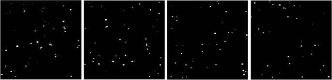

  

  The original image of settlement particles in the video 1

According to the weight calculation method in Section 4.2 and the relevant engineering data, the weights of the particle size and area of settling particles are 0.6 and 0.4, respectively, namely [0.6, 0.4]. The parameters of settlement particle membership function are set to d₁ = 5 and d₂ = 10, and the parameters of area membership function are set to S₁ = 25 and S₂ = 100.

• 2. Experimental results

The segmentation of the particle image is key to recognize the settlement particle, so we had used the different methods for the particle image segmentation by the Sobel operator, the normal region segmentation, and the proposed algorithm in video 1, whose results were respectively shown from Figs. 16, 17, and 18, respectively. Figure 18 shows the good segmentations prior to the other methods from the smoothness, sharpness, and brightness. Figure 19 is the settlement particle recognition result based on fuzzy comprehensive evaluation.

Fig. 16

Settlement particle image segmentation based on Sobel operator

Fig. 17

Settlement particle image based on region segmentation

Fig. 18

Segmentation result diagram of the method in this paper

Fig. 19

Settlement particle recognition based on fuzzy comprehensive evaluation

Figures 20 and 21 show the recognized large particles and the long tail particles in video 1, which were marked with a circle.

Fig. 20

The recognized large particles in the video 1

Fig. 21

The recognized long tail particles in the video 1

Figures 22 and 23 show the recognized large particles and the long tail particles in video 2, which were marked with a circle.

• 3. Experimental comparison

  Fig. 22

  

  Recognition results of large particles

  Fig. 23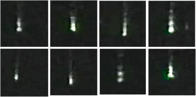

  

  Recognition results of long tail particles

For the comparison with the proposed methods, we did the experiments in video 1 by the classical Otsu threshold segmentation method, Gaussian mixture model, and Yang’s algorithm, and the results were shown in Figs. 24 and 25.

• 4. Analysis of experimental results

  Fig. 24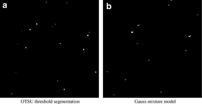

  

  The recognition results with Otsu threshold segmentation method and Gauss mixture model

  Fig. 25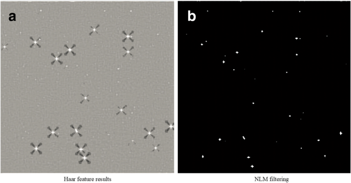

  

  Experimental results of Yang’s algorithm

The standard of settlement particle recognition algorithm is mainly measured by TPR and FPR, and its expression is like Eq. (27).

$$ TPR=\frac{TP}{TP+ FN},\kern2.75em FPR=\frac{FP}{FP+ TN}\kern7.25em $$

(27)

In Eq. (27), TP is the prediction result and the actual result are the number of settlement particles, FP is the prediction value is the settlement particle but the number of noise in fact, FN is the prediction value is the noise but in fact the number of settlement particles, TN is the prediction result, and the actual result are the number of noise. Figure 26 describes the ROC curves of each method and Table 1 describes the average time of each method.

Fig. 26

The ROC curves of each method

Table 1 Average time of each method

As can be seen from the above icons, the recognition accuracy of the proposed method is better than that of other algorithms, and from time, it is shorter than the Yang’s method, but it is a little longer than the Otsu algorithm and the Gauss mixture model. In summary, the algorithm in this paper has achieved good recognition results for settlement particles.

6 Conclusions

After the detail research on the settlement particle images and settlement particle sequence images, a multi-threshold segmentation method with the fuzzy 3-partitioning entropy is proposed, where the improved artificial bee colony algorithm is used to optimize the threshold, the recursive idea is also used to reduce the large number of repeated calculations in the fuzzy partitioning entropy, and the region-based label assignment method is applied to improve the accuracy of image segmentation. The experiment results show that the proposed algorithm has better segmentation performance.

References

J. Ma, H. Wen, X. Li, et al., Downy mildew diagnosis system for greenhouse cucumbers based on image processing. Nongye Jixie Xuebao/transactions of the Chinese Society of Agricultural Machinery 48(2), 195–202 (2017).
S. BS, E. LM, Particle tracking in drug and gene delivery research: state-of-the-art applications and methods. Adv. Drug Deliv. Rev. 91, 70–91 (2015).
G. Borgefors, On digital distance transforms in three dimensions. Comput. Vis. Image Underst. 64(3), 368–376 (1996).
G. Corkidi, U.R. Diaz, M.J. Folch, et al., COVASIAM: an image analysis method that allows detection of confluent microbial colonies and colonies of various sizes for automated counting. Appl. Environ. Microbiol. 64(4), 1400–1404 (1998).
P.K. Sethy, S. Panda, S.K. Behera, et al., On tree detection, counting & post-harvest grading of fruits based on image processing and machine learning approach-a review. International Journal of Engineering & Technology 9(2), 649–663 (2017).
Y. Tang, Y. Zhang, Y. Zhang, et al., A fast recursive algorithm based on fuzzy 2-partition entropy approach for threshold selection. Neurocomputing 74(17), 3072–3078 (2011).
H.C. Tsai, Y.H. Lin, Modification of the fish swarm algorithm with particle swarm optimization formulation and communication behavior. Appl. Soft Comput. 11(8), 5367–5374 (2011).
Z. Zhe, Research on cell sequence tracking method based on image segmentation[D], Jilin University (2017).
W.T. Wen, Research on rice quality detection system based on image processing[D], Jilin University (2015).
S. Benabdelkader, M. Boulemden, Recursive algorithm based on fuzzy 2-partition entropy for 2-level image thresholding. Pattern Recogn. 38(8), 1289–1294 (2005).
Y. Tang, W. Mu, Y. Zhang, et al., A fast recursive algorithm based on fuzzy 2-partition entropy approach for threshold selection. Neuro computing 74(17), 3072–3078 (2011).
Funding
The research is supported by the Science and Technology Basic Work Project “Investigation on Environmental Status of China’s Cement Industry” (2014FY110900) originated from Ministry of Science and Technology in China.
Availability of data and materials
Please contact author for data requests.
About the authors
Ran Zhou, software engineering, Master student in Wuhan University of Technology. His current research interests include data mining, artificial intelligence, image processing, and pattern recognition.
Huazhu Song, Doctor of Engineering, Associate Professor in Wuhan University of Technology. Her current research interests include data mining, artificial intelligence, machine learning, image processing, pattern recognition, semantic and ontology.
Jun Li, software engineering, software engineering, Master student in Wuhan University of Technology. His current research interests include data mining, artificial intelligence, and image processing.
Author information
Authors and Affiliations
Contributions
Three authors take part in the discussion of the work described in this paper. RZ researched on the topic of the paper and wrote the first version of the paper. HZS guided RZ’s research and modified the paper. JL helped to modify the figures in the paper and typeset the paper. All authors read and approved the final manuscript.
Corresponding author
Ethics declarations
Competing interests
The authors declare that they have no competing interests.
Publisher’s Note
Springer Nature remains neutral with regard to jurisdictional claims in published maps and institutional affiliations.
Rights and permissions
Open Access This article is distributed under the terms of the Creative Commons Attribution 4.0 International License (http://creativecommons.org/licenses/by/4.0/), which permits unrestricted use, distribution, and reproduction in any medium, provided you give appropriate credit to the original author(s) and the source, provide a link to the Creative Commons license, and indicate if changes were made.
About this article
Cite this article
Zhou, R., Song, H. & Li, J. Research on settlement particle recognition based on fuzzy comprehensive evaluation method. J Image Video Proc. 2018, 108 (2018). https://doi.org/10.1186/s13640-018-0344-0
Received:
Accepted:
Published:
DOI: https://doi.org/10.1186/s13640-018-0344-0