Double regularized matrix factorization for image classification and clustering

Abstract

Feature selection, which aims to select an optimal feature subset to avoid the “curse of dimensionality,” is an important research topic in many real-world applications. To select informative features from a high-dimensional dataset, we propose a novel unsupervised feature selection algorithm called Double Regularized Matrix Factorization Feature Selection (DRMFFS) in this paper. DRMFFS is based on the feature selection framework of matrix factorization, but extends this framework by introducing double regularizations (i.e., graph regularization and inner product regularization). There are three major contributions to our approach. First, for the sake of preserving the useful underlying geometric structure information of the feature space of the data, we introduce the graph regularization to guide the learning of the feature selection matrix, making it more effective. Second, in order to take into account the correlations among features, an inner product regularization term is imposed on the objective function of matrix factorization. Therefore, the selected features by DRMFFS cannot only represent the original high-dimensional data well but also contain low redundancy. Third, we design an efficient iteratively update algorithm to solve our approach and also prove its convergence. Experiments on six benchmark databases demonstrate that the proposed approach outperforms the state-of-the-art approaches in terms of both the classification and clustering performance.

1 Introduction

The dimensionality of the gathered data has been increasingly large due to the rapid development of modern sensing systems [1]. However, the high-dimensional data are hard to deal with since high computational complexity and memory requirements. Meanwhile, some irrelevant, redundant, and noisy features will be incorporated into high-dimensional data, which will adversely affect the performance. Hence, reducing the dimension of the data is an essential step for subsequent processing. Feature extraction [2, 3] and feature selection [4] can be regarded as two main techniques for dimensionality reduction. For feature extraction approaches, they obtain the features by mapping the original data into a new low-dimensional subspace using a transformation matrix or projection. Nevertheless, the obtained features have relatively poor interpretability [3]. In comparison, feature selection approaches aim at selecting several optimal features from the original data by a series of criteria [5]. Therefore, the obtained low-dimensional representation is interpretable [4]. More importantly, feature selection approaches just need to collect these optimal features during data acquisition, and they perform better than feature extraction approaches, which need to utilize all the features for dimensionality reduction. In this paper, we focus on feature selection.

Many feature selection approaches have been proposed in recent years. According to the availability of class label information, they can be categorized into three classes, including supervised feature selection [6], semi-supervised feature selection [7], and unsupervised feature selection [8, 9]. Supervised-based feature selection approaches search the optimal feature subset with the guidance of the class label information. However, in many real applications, there are small amount of labeled data or labeling all the data requires quite expensive human labor and computational costs. Therefore, supervised-based feature selection approaches are not feasible in the case of partially labeled data. Under this circumstance, a series of semi-supervised feature selection approaches have been designed, which take the information of the labeled and unlabeled data into account. Compared with the aforementioned feature selection techniques, unsupervised feature selection approaches determine an optimal feature subset, without any label information, and only depend on maintaining or revealing the intrinsic structures of the original data. Hence, how to incorporate the intrinsic structure information of the data into unsupervised feature selection is very critical.

A series of unsupervised feature selection approaches have been proposed. Among them, Variance Score (VS) might be the simplest unsupervised feature selection algorithm [10], which selects features based on their variance. After that, He et al. took advantage of locality-preservation ability of features and proposed an unsupervised feature selection approach called Laplacian Score (LS) [11]. The features selected by LS can maintain the manifold structure of the original data. In the sequel, Zhao and Liu combined the spectral graph theory into feature selection and presented Spectral Feature Selection (SPEC) [12]. In essence, VS, LS, and SPEC estimate the quality of features independently, ignoring the correlation among features.

In order to address the aforementioned issue, a series of sparsity regularization-based approaches have been presented [8, 9, 13,14,15,16,17,18,19,20,21,22,23] for unsupervised feature selection. For instance, Cai et al. presented Multi-Cluster Feature Selection (MCFS) [8] by combining spectral analysis (manifold learning) and sparse regression based on l₁-norm regularization. In MCFS, spectral analysis and sparse regression are two independent processes, and thereby, the effectiveness is degraded. To address such limitation, a series of studies which simultaneously perform the spectral analysis and sparse regression have been presented for unsupervised feature selection [9, 13,14,15,16,17,18,19,20,21,22,23]. Yang et al. proposed Unsupervised Discriminative Feature Selection (UDFS) [9] to select the most discriminative features for data representation. Similar to UDFS, Cong et al. proposed Unsupervised Deep Sparse Feature Selection (UDSFS) [13], which integrates the group sparsity of feature dimensions and feature units based on an l_{2, 1}-norm minimization into a unified framework to select the most discriminative features. Li et al. presented Nonnegative Discriminative Feature Selection (NDFS) [14], which performs non-negative spectral analysis and feature selection together. Yang et al. suggested Unsupervised Maximum Margin Feature Selection (UMMFSSC) [15]. In UMMFSSC, the clustering process and feature selection process are combined into a coherent framework to adaptively select the most discriminative subspace. Since the data always contain noise or outliers, Qian et al. proposed Robust Unsupervised Feature Selection (RUFS) [16] to address it, where robust clustering and robust feature selection are simultaneously performed by joint l_{2, 1}-norm minimization. Recently, self-representation property has been extensively utilized and many related approaches have been proposed [17]. In [18], Zhu et al. assumed that each feature can be represented as a linear combination of other features and proposed Regularized Self-Representation (RSR). Although good performance can be achieved by RSR, the structure preserving ability of features is neglected in it. To remedy it, a variety of extensions based on RSR have been put forward, i.e., Graph Regularized Nonnegative Self-Representation (GRNSR) [19] and Structure Preserving Nonnegative Feature Self-Representation (SPNFSR) [20]. Besides, Zhu et al. combined manifold learning and sparse regression together and proposed Joint Graph Sparse Coding (JGSC) [21]. In JGSC, a dictionary is firstly learned from the training data; then, the feature weight matrix can be obtained automatically via the learned dictionary. Since real-world data always contain lots of noise samples and features, the learned dictionary may be unrealizable to subsequent feature selection process [22]. Different from most of the aforementioned approaches which only utilize the geometric information of the data space, Shang et al. employed the manifold information of both the data space and the feature space simultaneously and proposed Non-Negative Spectral Learning with Sparse Regression-Based Dual-graph regularized feature selection (NSSRD) [23]. Through the experimental results in [23], it can be seen that the geometry information of the feature space plays a crucial role for further improving the quality of feature selection.

Apart from the above sparsity regularization-based unsupervised feature selection approaches, a series of matrix factorization-based approaches have been presented. Well-known examples of such methods include Principal Components Analysis (PCA) [24], Non-negative Matrix Factorization (NMF) [25], and Singular Value Decomposition (SVD) [26]. Nevertheless, these approaches are all designed for feature extraction rather than feature selection. Therefore, the low-dimensional features obtained by these approaches lack interpretability. To remedy this shortcoming, Wang et al. incorporated matrix factorization technique into the feature selection process and proposed a novel approach named Matrix Factorization based Feature Selection (MFFS) [27]. In MFFS, the feature selection can be regarded as the process of matrix factorization and the optimal feature subset is selected by introducing an orthogonality constraint into its objective function. Considering that MFFS conducts feature selection by integrating matrix factorization with an orthogonality constraint together, the orthogonality constraint is too strict to be satisfied in practice [23, 28, 29].

As previously mentioned, there are mainly two issues to these approaches. On the one hand, most of the state-of-the-art unsupervised feature selection approaches (e.g., LS, SPEC, MCFS, UDFS, UDSFS, NDFS, UMMFSSC, RUFS, GRNSR, SPNFSR, JGSC) can only take the geometric and discrimination information of the data space into consideration, while neglecting the useful underlying geometric structure information of the feature space during the process of dimensionality reduction [23]. Hence, some potentially valuable information is not fully exploited, reducing the performance of the algorithm. On the other hand, the majority of the existing approaches (e.g., MCFS, UDFS, UDSFS, NDFS, UMMFSSC, RUFS, RSR, GRNSR, SPNFSR, JGSC, and NSSRD) impose the l₁-norm regularization or l_{2, 1}-norm regularization on the feature weight matrix aiming to perform feature selection in a batch manner. Nevertheless, the l₁-norm or l_{2, 1}-norm neglect the redundancy measurement, so methods using l₁-norm regularization or l_{2, 1}-norm regularization might get into trouble when dealing with some informative but redundant features [30]. In general, the use of the l₁-norm or l_{2, 1}-norm regularization cannot achieve both sparsity and low redundancy simultaneously.

To address the above issues, this paper presents a novel approach called Double Regularized Matrix Factorization Feature Selection (DRMFFS) for conducting classification and clustering on high-dimensional data. Compared with the existing feature selection approaches, our main contributions lie in the following three-fold. First, to preserve the manifold information of the feature space, graph regularization which is a feature map constructed on the feature space, is imposed on the feature selection framework of matrix factorization. With the use of it, the learning of the coefficient matrix in error reconstruction term and the feature selection matrix can be guided. Therefore, it cannot only select a feature subset that can approximately represent the features, but also preserve the local geometrical information of the feature space. Second, to ensure the sparsity and low redundancy simultaneously, we introduce an inner product regularization term that can be regarded as a combination of the l₁-norm and l₂-norm on the objective function of matrix factorization. Third, a simple yet effective iteration update algorithm is proposed to optimize our model and a detailed analysis of its convergence is also given. Experiments on six databases, including Extended YaleB [31], CMU PIE [32], AR [33], JAFFE [34], ORL [35], and COIL20 [36] demonstrate that the proposed approach is effective.

The rest of this article is organized as follows: Section 2 presents the proposed method in detail. The experimental results and discussion are shown in Section 3. In the end, the conclusions are given in Section 4.

2 Methods

Firstly, the proposed DRMFFS model is given in detail. Secondly, we design an efficient iterative update algorithm to solve our model. Thirdly, we analyze its convergence. Finally, we compare the proposed approach with the related approaches to demonstrate its effectiveness. Table 1 gives some notation that is frequently used in this paper, which aims to facilitate the presentation.

Table 1 Some notation used in the paper

2.1 The DRMFFS model

Let X = [x₁; x₂; …; x _n ] ∈ R^n × dbe the high-dimensional unlabeled input data matrix, where n and d, respectively, represent the number and dimension of samples. The proposed approach aims to select a handful of optimal features that can approximately represent the entire set of features. Therefore, the distance between the spaces spanned by the original high-dimensional data samples and the selected features can be evaluated. According to [27], this problem can be converted into the following matrix factorization problem:

$$ {\displaystyle \begin{array}{l}\arg \underset{P,A}{\min }{\left\Vert X- XPA\right\Vert}_F^2\\ {}s.t.\kern0.8000001em P\ge 0\kern0.3em ,A\ge 0,{P}^TP={I}_{u\times u},\end{array}} $$

(1)

where A = [a₁, a₂, …, a _d ] ∈ R^u × d is the coefficient matrix used to project the original features into a new feature subspace spanned by the selected features, I_u × uis the u × u identity matrix, P = [p₁, p₂, p₃, …, p _d ]^T ∈ R^d × u denotes the feature weight matrix, and u denotes the count of the selected features. The constraint P^TP = I_u × u is used to ensure that the elements in P are ones or zeros. Here, we regard the matrix P as an indicator matrix of the selected features.

Although Eq. (1) can accomplish the feature selection task, there remain two drawbacks. First, the underlying geometric information of the feature space is neglected, which weakens the quality of feature selection. Second, the orthogonality constraint in Eq. (1) is too strict [23], which ignores the correlations among features.

Actually, local structure information plays an important role in feature selection. Therefore, many feature selection algorithms using local structure information have been proposed and achieve good performance. For example, Laplacian Score (LS) [11], Spectral Feature Selection (SPEC) [12], and Multi-Cluster Feature Selection (MCFS) [8] are three well-known algorithms. Meanwhile, some researchers have shown that the manifold information of the data is distributed not only in the data space but also in the feature space [37,38,39,40]. Therefore, the feature manifold also contains the underlying geometric structure information, which is beneficial for feature selection. Inspired by [37,38,39,40], we incorporate the local structure information of the feature space of the data into our algorithm to address the first shortcoming of Eq. (1). First, we build a k-nearest neighbor graph G = (V, E) based on the given sample matrix X. Here, each row vector of X corresponds to a feature, i.e., f _j is the jth feature of X. Then, we can rewrite X asX = [f₁; f₂; …; f _d ] ∈ R^d × n. For a graph G, we denote the set of feature points and the weights of the edges between the vertices, as V = [f₁, f₂, …, f _d ] and E = [E₁, E₂, …, E _d ], respectively. Specifically, we can regard the weight of the edge as the similarity between the two features, namely, the higher the weight, the more similar the features.

To ensure that the selected features retain the geometry information of the features in the original high-dimensional feature space, we can minimize the following equation:

$$ J=\arg \underset{A}{\min}\frac{1}{2}\sum \limits_{i=1}^d\sum \limits_{j=1}^d{\left\Vert {a}_i-{a}_j\right\Vert}_2^2{S}_{ij} $$

(2)

where a _i is the low-dimensional representation of f _i , and S _ij represents the similarity between features f _i and f _j , (i, j = 1, 2,…, d).

Since Gaussian heat kernel function is a simple and effective approach to discover the intrinsic geometrical structure of the data [3, 41, 42], this paper utilizes it to measure the closeness between features, which is defined as:

$$ {S}_{ij}=\left\{\begin{array}{cc}\exp \left(-{\left\Vert {f}_i-{f}_j\right\Vert}_2^2/{\sigma}^2\right),& if\kern0.3em {f}_i\in N\left({f}_j\right)\kern0.4em \mathrm{or}\kern0.3em {f}_j\in N\left({f}_i\right)\\ {}0& \mathrm{otherwise},\end{array}\right. $$

(3)

where N(f _i ) is the k-nearest neighbor set of feature f _i and σis a kernel parameter. If features f _i and f _j are close in the original high-dimensional feature space, the corresponding S _ij will be large, and vice versa.

By simple algebraic manipulation, Eq. (2) can be rewritten to:

$$ {\displaystyle \begin{array}{l}J=\arg \underset{A}{\min}\frac{1}{2}\sum \limits_{i=1}^d\sum \limits_{j=1}^d{\left\Vert {a}_i-{a}_j\right\Vert}_2^2{S}_{ij}\\ {}\kern0.9000001em =\arg \underset{A}{\min } tr\left(A\left(D-S\right){A}^T\right)\\ {}\kern1em =\arg \underset{A}{\min } tr\left({ALA}^T\right),\end{array}} $$

(4)

where D is a diagonal matrix and D _ii  = ∑ _j S _ij . The matrix L = D-S is the graph Laplacian matrix of feature space. According to Eq. (3), it is easy to see that if two features, e.g., f _i and f _j , are close to each other, then the similarity measurement S _ij is large. Actually, by minimizing Eq. (4), we tend to find such a matrix A that ensures that if the nearby features, e.g., f _i and f _j , are related to each other, and their corresponding low-dimensional representations, i.e., a _i and a _j , should still have the same and similar relations.

The second shortcoming of Eq. (1) is the strict orthogonality constraint. A straightforward way to address it is to introduce the existing regularization terms, such as the l₁-norm or l_{2, 1}-norm with respect to P in Eq. (1). Nevertheless, the characteristics of sparsity and low redundancy could not be achieved simultaneously [37] by these regularization terms. Recently, Han et al. designed a regularization term that can directly characterize the independence and saliency of variables [37]. Inspired by [37], in this paper, we utilize the absolute values of the inner product between feature weight vectors as the regularization term to relax the strict orthogonality constraint of Eq. (1), i.e., ∣ < p _i , p _j  > ∣, in which p _j  ∈ R^1 × u(j = 1, 2, …, d) is the jth row vector of P. Therefore, we can rewrite the regularization in our DRMFFS as:

$$ {\displaystyle \begin{array}{l}\Omega (P)=\sum \limits_{i=1}^d\sum \limits_{j=1,j\ne i}^d\mid <{p}_i,{p}_j>\mid \\ {}\kern2.95em =\sum \limits_{i=1}^d\sum \limits_{j=1}^d\mid <{p}_i,{p}_j>\mid -\sum \limits_{i=1}^d\mid <{p}_i,{p}_i>\mid \\ {}\kern2.95em =\sum \limits_{i=1}^d\sum \limits_{j=1}^d\mid <{p}_i,{p}_j>\mid -\sum \limits_{i=1}^d{\left\Vert {p}_i\right\Vert}_2^2.\end{array}} $$

(5)

Then, we rewrite the Eq. (5) as:

$$ {\displaystyle \begin{array}{l}\Omega (P)=\left({\left\Vert {PP}^T\right\Vert}_1- tr\left({P}^TP\right)\right)\\ {}\kern1.25em =\left({\left\Vert {PP}^T\right\Vert}_1-{\left\Vert P\right\Vert}_2^2\right).\end{array}} $$

(6)

Finally, we expect the metric in Eq. (6) to be as small as possible [37], and the weights that correspond to the redundant and uninformative features will be reduced to very small values or even zeros, which makes the feature selection more discriminative.

Next, through combining Eqs. (4) and (6) with the matrix factorization, the objective function of our DRMFFS algorithm can be obtained as:

$$ {\displaystyle \begin{array}{l}\underset{P,A}{\min }{\left\Vert X- XPA\right\Vert}_F^2+\upalpha \mathrm{tr}\left({\mathrm{ALA}}^T\right)+\beta \Omega (P)\\ {}=\underset{P,A}{\min }{\left\Vert X- XPA\right\Vert}_F^2+\upalpha \mathrm{tr}\left({\mathrm{ALA}}^T\right)+\beta \sum \limits_{i=1}^d\sum \limits_{j=1,j\ne i}^d\mid <{p}_i,{p}_j>\mid \\ {}s.t.\kern0.8000001em P\ge 0,\kern0.5em A\ge 0,\end{array}} $$

(7)

where α ≥ 0 and β ≥ 0 are two balance parameters. The first term measures the ability of the selected features; the second term aims at ensuring that the selected features can maintain the geometry structure information of the features in the original high-dimensional feature space; the third term is used to make the feature weight matrix sparse and of low redundancy.

By optimizing the proposed objective function, the feature weight matrix P = [p₁; p₂; …; p _d ] can be learned. Then, we can rank all the features in terms of ‖p _i ‖₂ in descending order and select the first u features to form the optimal feature subset.

2.2 Iterative updating algorithm

In Eq. (7), it contains two variables, i.e., P and A. Considering that Eq. (7) is not convex, we give an iterative update algorithm to optimize Eq. (7).

Let F(P, A) be the value of the objective function of Eq. (7), that is,

$$ {\displaystyle \begin{array}{l}F\left(P,A\right)={\left\Vert X- XPA\right\Vert}_F^2+\upalpha \mathrm{tr}\left({\mathrm{ALA}}^T\right)+\beta \sum \limits_{i=1}^d\sum \limits_{j=1,j\ne i}^d\mid <{p}_i,{p}_j>\mid \\ {}={\left\Vert X- XPA\right\Vert}_F^2+\upalpha \mathrm{tr}\left({\mathrm{ALA}}^T\right)+\beta \left({\left\Vert {PP}^T\right\Vert}_1-{\left\Vert P\right\Vert}_2^2\right)\\ {}s.t.\kern1em P\ge 0,A\ge 0.\end{array}} $$

(8)

After some algebraic manipulations, we can rewrite Eq. (8) as

$$ {\displaystyle \begin{array}{l}F\left(P,A\right)={\left\Vert X- XPA\right\Vert}_F^2+\upalpha \mathrm{tr}\left({\mathrm{ALA}}^T\right)+\beta \left({\left\Vert {PP}^T\right\Vert}_1\hbox{-} {\left\Vert P\right\Vert}_2^2\right)\\ {}= tr\left({\left(X\hbox{-} XPA\right)}^T\left(X\hbox{-} XPA\right)\right)+\upalpha \mathrm{tr}\left({\mathrm{ALA}}^T\right)\\ {}\kern5.599997em +\beta \left( tr\left({1}_{d\times d}{PP}^T\right)\hbox{-} tr\left({P}^TP\right)\right)\\ {}= tr\left({X}^TX\right)\hbox{-} 2 tr\left({A}^T{P}^T{X}^TX\right)+ tr\left({A}^T{P}^T{X}^T XPA\right)\\ {}\kern1em +\upalpha \mathrm{tr}\left({\mathrm{ALA}}^T\right)+\beta \left( tr\left({1}_{d\times d}{PP}^T\right)\hbox{-} tr\left({P}^TP\right)\right),\end{array}} $$

(9)

where 1_d × dis a d × d matrix with all the elements equal to 1.

Next, we introduce two Lagrange multipliers λ ∈ R^d × uand ϑ ∈ R^u × d to constrain P ≥ 0andA ≥ 0, respectively. So Eq. (9) can be rewritten as Lagrange’s function:

$$ {\displaystyle \begin{array}{l}L\left(F,\lambda, \vartheta \right)=F\left(P,A\right)+ tr\left(\lambda P\right)+ tr\left(\vartheta A\right)\\ {}\kern0.3em = tr\left({X}^TX\right)-2 tr\left({A}^T{P}^T{X}^TX\right)\\ {}\kern0.7em + tr\left({A}^T{P}^T{X}^T XPA\right)+\alpha tr\left({ALA}^T\right)+\beta \Big( tr\left({1}_{d\times d}{PP}^T\right)\\ {}\kern1em - tr\left({P}^TP\right)\Big)+ tr\left(\lambda P\right)+ tr\left(\vartheta A\right).\end{array}} $$

(10)

By taking the derivatives of Eq. (10) with respect to P and A, and setting them equal to zero, we get:

$$ \frac{\partial L}{\partial P}=-2{X}^T{XA}^T+2{X}^T{XPAA}^T+2\beta \left({1}_{d\times d}P-P\right)+\lambda =0 $$

(11)

$$ \frac{\partial L}{\partial A}=-2{P}^T{X}^TX+2{P}^T{X}^T XPA+2\alpha A\left(D-S\right)+\vartheta =0. $$

(12)

Using the Karush-Kuhn-Tucker (KKT) [43] conditions λ _ij P _ij  = 0 and ϑ _ji A _ji  = 0, we obtain:

$$ {P}_{ij}\leftarrow {P}_{ij}\frac{{\left({X}^T{XA}^T+\beta P\right)}_{ij}}{{\left({X}^T{XPAA}^T+\beta {1}_{d\times d}P\right)}_{ij}}, $$

(13)

$$ {A}_{ji}\leftarrow {A}_{ji}\frac{{\left({P}^T{X}^TX+\alpha AS\right)}_{ji}}{{\left({P}^T{X}^T XPA+\alpha AD\right)}_{ji}}. $$

(14)

The whole procedure of our algorithm is summarized in Algorithm 1. First, we need to calculate the similarity matrix among features, whose computation complexity is Ο(d²n). Then, the time complexity of each iteration in Algorithm 1 is equal to Ο(u²d + nd² + ud²). Note that the number of the selected features u is smaller than the number of original features d. So, the total time complexity of our algorithm equals to Ο(Tnd²), in which T is the number of iterations.

2.3 Convergence analysis

The convergence of the update criteria in Eqs. (13) and (14) are given as follows:

Theorem 1.

ForP ≥ 0, A ≥ 0, the value of the objective function in Eq. (8) is non-increasing and has a lower boundary under the update rules in Eq. (13) and Eq. (14).

Here, we incorporate an auxiliary function to prove Theorem 1, which is defined as follows:

Definition 1.

ϕ(v, v^') is an auxiliary function of ψ(v) if conditions ϕ(v, v^') ≥ ψ(v)and ϕ(v, v) = ψ(v) are satisfied [25].

The auxiliary function is very useful because of the following lemma:

Lemma 1.

Suppose that ϕ is an auxiliary function of ψ; then, ψis non-increasing under the following update rule:

$$ {v}^{\left(t+1\right)}=\arg \underset{v}{\min}\phi \left(v,{v}^{(t)}\right), $$

(15)

where t indicates the tth iteration.

Proof ψ(v^(t + 1)) ≤ ϕ(v^(t + 1), v^(t)) ≤ ϕ(v^(t), v^(t)) = ψ(v^(t)).□

First, it is necessary to prove that the update criterion for P in Eq. (13) is consistent with Eq. (15) when an auxiliary function is properly designed. We defineψ _ij (P _ij )as the part of Eq. (8) that is only related toP _ij . Therefore, we have:

$$ {\displaystyle \begin{array}{l}{\psi}_{ij}\left({P}_{ij}\right)=\Big(-2{A}^T{P}^T{X}^TX+{A}^T{P}^T{X}^T XPA\\ {}\kern7.399995em +\beta {1}_{d\times d}{PP}^T-\beta {P}^TP\Big){}_{ij},\end{array}} $$

(16)

$$ {\displaystyle \begin{array}{l}\nabla {\psi}_{ij}\left({P}_{ij}\right)=\Big(-2{X}^T{XA}^T+2{X}^T{XPAA}^T\\ {}\kern7.099996em +2\beta {1}_{d\times d}P-2\beta P\Big){}_{ij},\end{array}} $$

(17)

$$ {\nabla}^2{\psi}_{ij}\left({P}_{ij}\right)=2{\left({X}^TX\right)}_{ii}{\left({A}^TA\right)}_{jj}+2\beta {\left({1}_{d\times d}-I\right)}_{ii}, $$

(18)

where ∇ψ _ij (P _ij ) and ∇²ψ _ij (P _ij ) represent the first-order and second-order derivatives, respectively, of the objective function ψ _ij with respect toP _ij .

Lemma 2.

The function in Eq. (19) is a reasonable auxiliary function of ψ _ij (P _ij ).

$$ {\displaystyle \begin{array}{l}\phi \left({P}_{ij},{P}_{ij}^{(t)}\right)={\psi}_{ij}\left({P}_{ij}^{(t)}\right)+\nabla {\psi}_{ij}\left({P}_{ij}^{(t)}\right)\left({P}_{ij}-{P}_{ij}^{(t)}\right)\\ {}\kern5.099998em +\frac{{\left({X}^T{\mathrm{XPAA}}^T+\beta {1}_{d\times d}P\right)}_{ij}}{P_{ij}^{(t)}}{\left({P}_{ij}-{P}_{ij}^{(t)}\right)}^2.\end{array}} $$

(19)

Proof Through the Taylor series expansion of ψ _ij (P _ij ), we obtain:

$$ {\displaystyle \begin{array}{l}{\psi}_{ij}\left({P}_{ij}\right)={\psi}_{ij}\left({P}_{ij}^{(t)}\right)+\nabla {\psi}_{ij}\left({P}_{ij}^{(t)}\right)\left({P}_{ij}-{P}_{ij}^{(t)}\right)\\ {}\kern3.699999em +\frac{1}{2}{\nabla}^2{\psi}_{ij}\left({P}_{ij}^{(t)}\right){\left({P}_{ij}-{P}_{ij}^{(t)}\right)}^2\\ {}\kern2.999999em ={\psi}_{ij}\left({P}_{ij}^{(t)}\right)+\nabla {\psi}_{ij}\left({P}_{ij}^{(t)}\right)\left({P}_{ij}-{P}_{ij}^{(t)}\right)\\ {}\kern3.899998em +\left\{{\left({X}^TX\right)}_{ii}{\left({A}^TA\right)}_{jj}+\beta {\left({1}_{d\times d}-I\right)}_{ii}\right\}{\left({P}_{ij}-{P}_{ij}^{(t)}\right)}^2.\end{array}} $$

(20)

Through integrating Eq. (19) with Eq. (20), we can learn that $\phi \left({P}_{ij},{P}_{ij}^{(t)}\right)\ge {\psi}_{ij}\left({P}_{ij}\right)$ is equivalent to:

$$ \frac{{\left({X}^T{\mathrm{XPAA}}^T+\beta {1}_{d\times d}P\right)}_{ij}}{P_{ij}^{(t)}}\ge {\left({X}^TX\right)}_{ii}{\left({A}^TA\right)}_{jj}+\beta {\left({1}_{d\times d}-I\right)}_{ii}. $$

(21)

In according with linear algebra, we can obtain:

$$ {\displaystyle \begin{array}{l}{\left({X}^T{\mathrm{XPAA}}^T\right)}_{ij}=\sum \limits_{l=1}^u{\left({X}^T{XP}^{(t)}\right)}_{il}{\left({A}^TA\right)}_{lj}\ge {\left({X}^T{XP}^{(t)}\right)}_{ij}{\left({A}^TA\right)}_{jj}\\ {}\kern6.599996em \ge \sum \limits_{l=1}^d{\left({X}^TX\right)}_{il}{P}_{lj}^{(t)}{\left({AA}^T\right)}_{jj}\\ {}\kern6.599996em \ge {\left({X}^TX\right)}_{ii}{P}_{ij}^{(t)}{\left({AA}^T\right)}_{jj}={P}_{ij}^{(t)}{\left({X}^TX\right)}_{ii}{\left({AA}^T\right)}_{jj}.\end{array}} $$

(22)

$$ \beta {\left({1}_{d\times d}P\right)}_{ij}=\beta \sum \limits_{l=1}^d{\left({1}_{d\times d}\right)}_{il}{P}_{lj}^{(t)}\ge \beta \sum \limits_{l=1}^d{\left({1}_{d\times d}-I\right)}_{il}{P}_{lj}^{(t)}\ge \beta {\left({1}_{d\times d}-I\right)}_{ii}{P}_{ij}^{(t)}. $$

(23)

From Eqs. (22) and (23), we observe that Eq. (21) holds and $\phi \left({P}_{ij},{P}_{ij}^{(t)}\right)\ge {\psi}_{ij}\left({P}_{ij}\right)$. In addition, $\phi \left({P}_{ij},{P}_{ij}^{(t)}\right)={\psi}_{ij}\left({P}_{ij}\right)$ is obvious. Thus, Lemma 2 is proved. □

Next, we employ the similar method as that described above to analyze the variable A. We use ψ _ji (A _ji ) to denote the part of Eq. (8) and obtain:

$$ {\psi}_{ji}\left({A}_{ji}\right)={\left(-2{A}^T{P}^T{X}^TX+{A}^T{P}^T{X}^T XPA+2\alpha {ALA}^T\right)}_{ji} $$

(24)

$$ \nabla {\psi}_{ji}\left({A}_{ji}\right)={\left(-2{P}^T{X}^TX+2{P}^T{X}^T XPA+2\alpha AL\right)}_{ji} $$

(25)

$$ {\nabla}^2{\psi}_{ji}\left({A}_{ji}\right)=2{\left({P}^T{X}^T XP\right)}_{jj}+{(L)}_{ii} $$

(26)

where ∇ψ _ji (A _ji ) and ∇²ψ _ji (A _ji ) represent the first-order and second-order derivatives of ψ _ji with respect to A _ji .

Lemma 3.

The following function in Eq. (27) is a reasonable auxiliary function of ψ _ji (A _ji ).

$$ {\displaystyle \begin{array}{l}\phi \left({A}_{ji},{A_{ji}}^{(t)}\right)={\psi}_{ji}\left({A_{ji}}^{(t)}\right)+\nabla {\psi}_{ji}\left({A_{ji}}^{(t)}\right)\left({A}_{ji}-{A_{ji}}^{(t)}\right)\\ {}\kern6.199996em +\frac{{\left({P}^T{X}^T XPA+ AD\right)}_{ji}}{{A_{ji}}^{(t)}}{\left({A}_{ji}-{A_{ji}}^{(t)}\right)}^2.\end{array}} $$

(27)

Proof Through the Taylor series expansion of ψ _ji (A _ji ), we obtain:

$$ {\displaystyle \begin{array}{l}\psi \left({A}_{ji}\right)={\psi}_{ji}\left({A_{ji}}^{(t)}\right)+\nabla {\psi}_{ji}\left({A_{ji}}^{(t)}\right)\left({A}_{ji}-{A_{ji}}^{(t)}\right)\\ {}\kern4.199998em +\frac{1}{2}{\nabla}^2{\psi}_{ji}\left({A_{ji}}^{(t)}\right){\left({A}_{ji}-{A_{ji}}^{(t)}\right)}^2\\ {}\kern2.7em ={\psi}_{ji}\left({A_{ji}}^{(t)}\right)+\nabla {\psi}_{ji}\left({A_{ji}}^{(t)}\right)\left({A}_{ji}-{A_{ji}}^{(t)}\right)\\ {}\kern4.099998em +\left\{{\left({P}^T{X}^T XP\right)}_{jj}+{L}_{ii}\right\}{\left({A}_{ji}-{A_{ji}}^{(t)}\right)}^2.\end{array}} $$

(28)

Through comparing Eq. (27) with Eq. (28), it is easy to see that ϕ(A _ji , A _ji ^(t)) ≥ ψ _ji (A _ji )equals to:

$$ \frac{{\left({P}^T{X}^T XP A+ AD\right)}_{ji}}{{A_{ji}}^{(t)}}\ge {\left({P}^T{X}^T XP\right)}_{jj}+{L}_{ii}. $$

(29)

In according with the linear algebra, we obtain:

$$ {\left({P}^T{X}^T XP A\right)}_{ji}=\sum \limits_{l=1}^u{\left({P}^T{X}^T XP\right)}_{jl}{A}_{li}^{(t)}\ge {\left({P}^T{X}^T XP\right)}_{jj}{A}_{ji}^{(t)}. $$

(30)

$$ {(AD)}_{ji}=\sum \limits_{l=1}^u{A}_{jl}^{(t)}{D}_{li}\ge {A}_{ji}^{(t)}{D}_{ii}={A}_{ji}^{(t)}{D}_{ii}\ge {A}_{ji}^{(t)}\left({D}_{ii}-{S}_{ii}\right)={A}_{ji}^{(t)}L{}_{ii}. $$

(31)

From Eqs. (30) and (31), we know that Eq. (29) holds and ϕ(A _ji , A _ji ^(t)) ≥ ψ _ji (A _ji ). Considering that we can check ϕ(A _ji , A _ji ^(t)) = ψ _ji (A _ji ) easily, Lemma 3 is proved. □.

Finally, we will give a proof of the convergence of Theorem 1.

Proof of Theorem 1 we use the auxiliary function in Eq. (19) to replace ϕ(v, v^(t)) in Eq. (15) and obtain:

$$ {\displaystyle \begin{array}{l}{P}_{ij}^{\left(t+1\right)}={P}_{ij}^{(t)}-{P}_{ij}^{(t)}\frac{\nabla {\psi}_{ij}\left({P}_{ij}^{(t)}\right)}{2{\left({X}^T{\mathrm{XPAA}}^T+\beta {1}_{d\times d}P\right)}_{ij}}\\ {}\kern2.1em ={P}_{ij}^{(t)}\frac{{\left({X}^T{XA}^T+\beta P\right)}_{ij}}{{\left({X}^T{\mathrm{XPAA}}^T+\beta {1}_{d\times d}P\right)}_{ij}}.\end{array}} $$

(32)

Likewise, we utilize the auxiliary function in Eq. (27) to replace ϕ(v, v^(t)) in Eq. (15) and obtain:

$$ {\displaystyle \begin{array}{l}{A}_{ji}^{\left(t+1\right)}={A}_{ji}^{(t)}-{A}_{ji}^{(t)}\frac{\nabla {\psi}_{ji}\left({A}_{ji}^{(t)}\right)}{2{\left({P}^T{X}^T\mathrm{XPA}+\alpha AD\right)}_{ji}}\\ {}\kern2.6em ={A}_{ji}^{(t)}\frac{{\left({P}^T{X}^TX+\alpha AS\right)}_{ji}}{{\left({P}^T{X}^T\mathrm{XPA}+\alpha AD\right)}_{ji}}.\end{array}} $$

(33)

Since Eqs. (19) and (27) are the auxiliary functions of ψ _ij , ψ _ij is non-increasing under the update criteria in Eqs. (13) and (14). Lastly, considering that all of the terms in Eq. (8) are non-negative, the objective function of the proposed DRMFFS approach has a lower bound. Hence, in accordance with Cauchy’s convergence rule [44], the proposed model is convergent. □

2.4 Comparison with other approaches

In this subsection, we will highlight the effectiveness of our DRMFFS from the following two aspects:

• (1) We compare our DRMFFS with the related unsupervised feature selection approaches including LS, SPEC, MCFS, UDSFS, RUFS, RSR, SPNFSR, JGSC, NSSRD, and MFFS. Firstly, different from most of the existing unsupervised feature selection approaches, such as LS, SEPC, MCFS, UDSFS, RUFS, SPNFSR, and JGSC that consider the manifold information of the data space, our DRMFFS utilizes the graph regularization to directly preserve the local structure information of the feature space, which can provide more accurate discrimination information for feature selection. Secondly, for sparsity regularization-based unsupervised feature selection approaches, such as MCFS, UDSFS, RUFS, RSR, SPNFSR, JGSC, and NSSRD, they select a subset of features based on the l₁-norm or l_{2, 1}-norm. However, these approaches except UDSFS ignore the correlation among features, and thereby, the features selected by them may contain some redundancy, which makes the feature subset far from optimal. In contrast, our approach employs the absolute values of the inner product of the feature weight matrix vectors as a regularization term to ensure that the feature subset contains sparsity and low redundancy simultaneously. Finally, in comparison with Matrix Factorization-Based Feature Selection approach, i.e., MFFS, our DRMFFS uses the inner product constraint term in place of the strict orthogonality constraint term making our approach more flexible and effective.

• (2) We utilize the visualization of the features selected by different approaches to further demonstrate the effectiveness of our DRMFFS. First, we randomly select three sample images with the size of 32 × 32 pixels from three different face databases, i.e., ORL, AR, and CMU PIE. Then, all the approaches are applied to them and the selected features are labeled on this image. Here, the number of the selected features is fixed as 100 for all of the approaches. Figure 1 illustrates the corresponding experimental results, in which red color is used to represent the selected features and the features which are not selected retain the original gray. As seen from Fig. 1, all of the approaches except our DRMFFS select the features from uninformative parts of the face, such as the forehead and cheek or evenly distributed on the face. On the contrary, our DRMFFS can select the most representative face features, such as the eyes, eyebrows, nose, and mouth. Actually, observing Fig. 1, we can find two interesting phenomena as follows. On the one hand, the features selected by DRMFFS mostly focus on the recognizable parts of the face (i.e., eyes, eyebrows, nose, and mouth). The main reason is that our DRMFFS uses the graph regularization to preserve the geometric structure information on the feature manifold, making the selected features more holistic and structural. On the other hand, the selected features which are used to represent the eyes, mouth, and nose are mainly from the one side of the face. This phenomenon is due to the fact that DRMFFS takes the correlations among features into consideration, and thereby, the selected features are mainly from one side of the nearly symmetrical face components, accomplishing the low-redundancy.

  Fig. 1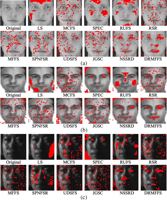

  

  The visualization results of selected features by different approaches on three different databases. a A sample image coming from ORL. b A sample image coming from AR. c A sample image coming from CMU PIE

Besides, we randomly select a sample image from Extended YaleB database as the experimental sample and apply our DRMFFS to this sample. Figure 2 shows the visualization result of our approach under different number of selected features. In Fig. 2, the red color is used to represent the selected features and the features which are not selected retain the original gray. Here, the number of selected features is tuned from {20, 50, 100, 150, 200, 250, 300}. Seen from Fig. 2, when the number of selected features is relatively small, the outline of the human face is not clear since the selected features rarely locate on the recognizable parts of the face. However, with the increase in number of selected features (from left to right), the extracted face information is also increased. In other words, our DRMFFS fails to select the most representative features such as the mouth and nose when the number of selected features is relatively small. The reason for the degraded performance of our DRMFFS under less number of features is that our approach utilizes the distance between the spaces spanned by the original high-dimensional data samples and the selected features as the evaluation criterion (see Eq. (1)). Therefore, when considering smallest features to be selected, the space spanned by our approach cannot well approximate the space spanned by original input samples, which leads to the information of high-dimensional data cannot be sufficiently maintained.

Fig. 2

The visualization result of our DRMFFS under different number of selected features

3 Results and discussion

In this section, we will carry out classification and clustering experiments to verify the effectiveness of the proposed approach in comparison with other state-of-the-art approaches.

3.1 Database

In our experiment, we use six benchmark image databases, including Extended YaleB [31], CMU PIE [32], AR [33], JAFFE [34], ORL [35], and COIL20 [36], to compare the performance of our approach with those of the state-of-the-art unsupervised feature selection approaches. Detailed descriptions of the six databases are given in Table 2, and some image examples from these databases are shown in Fig. 3.

• (1) Extended YaleB [31]: it consists of 2414 facial images from 38 persons. Each person has 64 images, and each image is cropped to the size of 32 × 32 pixels with 256 Gy levels per pixel. Some face images from the Extended YaleB database are depicted in Fig. 3a.

• (2) CMU PIE [32]: it includes 41,368 face images of 68 persons. In our experiment, we choose a subset (C29) that contains 210 face images of 10 persons from this dataset. Example images are shown in Fig. 3b.

• (3) AR face [33]: it consists of 4000 facial images that depict 126 distinct subjects (70 male and 56 female faces). The images of each subject were taken in varying conditions. The example images are shown in Fig. 3c.

• (4) JAFFE [34]: there are 213 facial images in it. Each person has seven different kinds of facial expressions. The example images from AR are given in Fig. 3d.

• (5) ORL [35]: there are ten different images of each of 40 distinct subjects. For each subject, the images were taken at different times, varying the lighting conditions. The example images from ORL are depicted in Fig. 3e.

• (6) COIL20 [36]: it is a database of gray-scale images of 20 objects. Each of subjects has 72 images, which were taken at pose intervals of 5° to vary object pose with respect to a xed camera. The example images from this database are illustrated in Fig. 3f.

Table 2 Statistics of the six databases

Fig. 3

Some of the images from different databases. a Extended YaleB. b CMU PIE. c AR. d JAFFE. e ORL. f COIL20

3.2 Experimental settings

In our experiments, we choose ten representative unsupervised feature selection algorithms as the comparison approaches. The ten comparison approaches include LS [11], MCFS [8], SPEC [12], UDSFS [13], RUFS [16], RSR [18], SPNFSR [20], JGSC [21], NSSRD [23], and MFFS [27]. Meanwhile, several details for the experiment parameter setting are as follows. For LS, MCFS, SPEC, UDSFS, SPNFSR, JGSC, NSSRD, and our approach, we fix the number of neighborhoods to 5 on all the databases. For UDSFS, RUFS, RSR, SPNFSR, JGSC, and NSSRD, the sparsity parameters will be tuned by a grid-search strategy from{10⁻³, 10⁻², 10⁻¹, 10⁰, 10¹, 10², 10³}. Following [27], we fix the value of the parameter in MFFS to 10⁸. For DRMFFS, we exploit the parameters α and β in the range of {0,   10⁰, 10¹, 10², 10³, 10⁴, 10⁵} on all the databases. We will report the best results obtained from the optimal parameters for all the approaches.

3.3 Classification results and analysis

In this subsection, we perform six different experiments on three databases including the Extended YaleB, CMU PIE, and AR to verify the effectiveness of our approach.

In the first experiment, we choose randomly l (l = 20, 12, 7) images per class for training from each of the three databases and reserve the remaining images for testing. The process is repeated 10 times, and the average classification accuracies and standard deviations of different approaches are reported in Table 3. Since the experiment environment and setting are the same with our previous paper [19]. Hence, a part of experimental results of the comparison approaches are directly from our previous work [19]. The number in parentheses is the number of the selected features that corresponds to the best result. Analyzing Table 3, it is obvious that all the feature selection approaches except LS outperform the baseline approach, which indicates that feature selection is an important and indispensable measure to remove the noise and redundant features of the data and to improve the classification performance. Besides, LS and SPEC conduct feature selection in a one-by-one manner. In contrast to LS and SPEC, the approaches MCFS, RUFS, MFFS, RSR, SPNFSR, UDSFS, JGSC, NSSRD, and our approach select the features jointly and achieve good performances. Specially, our DRMFFS achieves the best performance on all the three databases, compared with all the compared approaches. Moreover, the superiority of our DRMFFS over the newest approaches, i.e., JGSC, UDSFS, and NSSRD, also demonstrates that the combination of graph regularization and inner product regularization is crucial to select the most informative features from high-dimensional data.

Table 3 The average recognition rates and standard deviations of different algorithms on different databases. The best results are highlighted in italics

In the second experiment, the impact of different numbers of the selected features on the performance of our DRMFFS is tested. In this experiment, the number of the selected features is tuned by a grid-search strategy from{10, 20, 30, 40, …, 480, 490, 500}. Figure 3 illustrates the classification results of all the compared approaches on the Extended YaleB, CMU PIE, and AR databases with different numbers of the selected features. Seen from Fig. 4, the recognition rates of all the algorithms are improved at the beginning with an increase in the number of the selected features. However, this trend changes after they achieve their best performances. Besides, we can find that the performances of matrix factorization-based approaches including MFFS and our DRMFFS are inferior to some other methods when the number of selected features is relatively small. The main reason may lie in that the space spanned by only a small number of features cannot approximate the space spanned by original input samples. Thus, the information of high-dimensional data is not sufficiently maintained.

Fig. 4

a–c The recognition rates (%) of different feature selection algorithms on three different databases

In the third experiment, the influence of two regularization parameters (i.e., α and β) on the performance of our DRMFFS is evaluated. We first set the same initialization for different parameters and then test the impact of varying the values of parameters α and β on the performance of the proposed approach. Figure 5 depicts the classification results on three databases under different values of α and β. As shown in Fig. 5, the classification results of the proposed approach change little under different values of α and β on all the databases, which indicates that our approach is insensitive to the choice of parameters α and β. The average recognition rates obtained by our DRMFFS are 0.7277 ± 0.0086 (290), 0.9233 ± 0.0105 (250), and 0.7040 ± 0.0115 (300) for the Extended YaleB, CMU PIE, and AR databases, respectively, which are higher than the results obtained by the newest approaches, i.e., NSSRD, JGSC, and JGSC, which are listed in Table 3. These results indicate that incorporating both the geometric structure information of the feature space and the correlation among features together are of great importance for feature selection, which can improve the classification performance. Meanwhile, when the value of β is set to zero and α is set to a non-zero value, the recognition rates obtained by DRMFFS are relatively higher than those obtained when setting α to zero. Specially, when the value of α is set to zero, our approach is inferior to those obtained under other non-zero settings since the local structure information of the feature space of the data is totally neglected. Therefore, the preserving of the local structure information of the feature space of the data is important for feature selection. In addition, a relatively large α value or a relatively small β value will cause the second term of the objective function in (7) to dominate and overlook the other two terms. A relatively large β value or a relatively small α value will cause the third term of the objective function in (7) to dominate, and both the matrix factorization and the local structure information of the feature space of the data will be neglected. All in all, the proposed approach can achieve its best performance when the values of α and β are neither too large nor too small. Moreover, we also can see that the varied performances are not caused by different initializations, but the constraints that the initial settings are the same for varied parameters.

Fig. 5

a–c The recognition rates (%) of DRMFFS vs. parameters α and β on three different databases

In the fourth experiment, we test the influence of initialization for our approach by randomly selecting a set of training samples and testing samples from the AR, Extended YaleB, and CMU PIE databases. Meanwhile, we set the parameters of the algorithm as the optimal parameters. In this test experiment, we randomly generate the matrices A and P, then calculate the recognition rate of the algorithm. Here, the random generation process is repeated 30 times and the corresponding result is shown in Fig. 6. As seen from Fig. 6, the recognition rate of our approach is relatively stable at different initializations. Also, it demonstrates that our approach is insensitive to different initializations. The main reason is that our approach eventually converges under different initializations.

Fig. 6

The recognition rates (%) of DRMFFS vs. varying random initialization generation processes on three databases

In the fifth experiment, we utilize the one-tailed t test to further verify whether DRMFFS performs significantly better than other approaches. In this test, the null hypothesis is that our DRMFFS makes no difference when compared to the existing unsupervised feature selection approaches in classification task and the alternative hypothesis is that our DRMFFS makes an improvement when compared to the other approaches. For example, if we want to compare the performance of DRMFFS with that of JGSC (DRMFFS vs. JGSC), the null and alternative hypotheses are defined as H₀ : M_DRMFFS = M_JGSC andH₁ : M_DRMFFS > M_JGSC, respectively, where M_DRMFFS and M_JGSCare the average classification results obtained by DRMFFS and JGSC approaches on all of the three databases in Section 3.3. In our experiment, the significance level is set to 0.05. As seen from the test results depicted in Table 4, the p values obtained by all the pairwise t tests are much less than 0.05, which means that the null hypotheses are disapproved in all the pair-wise t tests. Therefore, the proposed approach significantly outperforms other approaches.

Table 4 The p values of the pairwise one-tailed t tests of DRMFFS and other approaches on classification accuracy

Finally, the convergence curves of the proposed approach on three different databases are shown in Fig. 7. As seen from these figures, the proposed approach converges very fast on all the databases, which demonstrates the efficiency and effectiveness of the proposed optimal approach.

Fig. 7

a–c Convergence curves of DRMFFS on three different databases

3.4 Clustering results and analysis

In the clustering experiments, two widely used criteria, i.e., clustering accuracy (ACC) and normalized mutual information (NMI) are adopted to compare the clustering performances of different unsupervised feature selection approaches. The larger ACC or NMI is, the better the performance of the algorithm, and vice versa. Given an input sample x _i , let c _i and g _i be its clustering label and ground-truth label. The ACC can be formulated as

$$ \mathrm{ACC}=\frac{\sum \limits_{i=1}^n\gamma \left({g}_i,\mathrm{map}\left({c}_i\right)\right)}{n} $$

(34)

where γ(g _i , c _i ) denotes an indicator function that equals 1 if c _i  = g _i and equals 0 if c _i  ≠ g _i . Here,map(⋅) is the optimal mapping function that maps each clustering label to an equivalent true label by the Kuhn-Munkres algorithm [45].

NMI is defined as:

$$ \mathrm{NMI}\left(Q,R\right)=\frac{I\left(Q,R\right)}{\sqrt{H(Q)H(R)}} $$

(35)

where I(Q, R) represents the mutual information of Q and R; the entropies of Q and R are, respectively, denoted as H(Q) and H(R). In this study, Q and R are the clustering label and the ground-truth, respectively.

According to the selected features, we utilize the k-means algorithm to cluster all the samples, by different feature selection algorithms. Considering that the performance of the k-means clustering approach relies on the initialization, we repeat the process of clustering 50 times with different random initializations and the average clustering results with standard deviations are given for this experiment. In this subsection, we use JAFFE, ORL, and COIL20 databases to evaluate the effectiveness of the proposed approach in terms of ACC and NMI.

First, we tune the number of the selected features from 10 to 500 with an interval of 10 to test the clustering performance of different approaches. Tables 5 and 6 report the best ACC and NMI from the optimal fixed parameters obtained by different approaches. In Tables 5 and 6, the number in parentheses is the number of the selected features that corresponds to the best clustering result. Since we use the same clustering experiment parameter setting with our previous work [21], the clustering results of some compared approaches are the same with [21]. Several interesting points can be observed from Tables 5 and 6. First, all the feature selection approaches outperform than the baseline algorithm, indicating that feature selection plays an important role for clustering. Second, both LS and SPEC independently select features without considering the correlations among features. Therefore, their clustering performances are inferior to those of the sparsity regularized-based approaches (i.e., MCFS, RUFS, RSR, SPNFSR, UDSFS, JGSC, NSSRD) and matrix factorization theory-based approaches (i.e., MFFS and our DRMFFS) on all the databases. This indicates that they select the features in a batch manner which is more effective than individually. Although these approaches jointly select features and achieve better performance than LS and SPEC, they either ignore the geometric structure information of the feature space (i.e., MCFS, RUFS, SPNFSR, RSR, UDSFS, JGSC, MFFS), or the correlations among features (i.e., MCFS, RUFS, SPNFSR, RSR, JGSC, MFFS, NSSRD), which will greatly reduce the effectiveness of feature selection. Finally, it can be seen that our DRMFFS outperforms the competing approaches. That is because the DRMFFS takes the geometric structure information of the feature space into the process of feature selection, making the selected feature subset more accurate. Furthermore, the DRMFFS has more advantages than the sparsity regularized-based approaches by replacing the l₁-norm or l₂-norm with the inner product regularization term that can be regarded as a combination of the l₁-norm and l₂-norm, such as considering the correlations among features, achieving sparsity, and low redundancy simultaneously. All in all, our approach can achieve the best performance on all the databases, which demonstrates that the proposed approach is effective.

Table 5 Clustering results (ACC ± std) of different approaches on three different databases. The best results are highlighted in italics

Table 6 Clustering results (NMI ± std) of different approaches on three different databases. The best results are highlighted in italics

Second, the impact of various numbers of the selected features on the clustering performance (i.e., ACC and NMI) of different approaches is tested and the results are shown in Figs. 8 and 9. From the two figures, we can also observe that the clustering performances of our approach are inferior to those of some other approaches when the number of the selected features is small. The reason is the same as the classification experiments. However, with an increase of selected features, the proposed approach performs excellent and is finally superior to all the compared approaches at higher dimensions.

Fig. 8

a–c The ACC (%) of different feature selection algorithms on three different databases

Fig. 9

a–c The NMI (%) of different feature selection algorithms on three different databases

Next, similar to the classification experiment, we test the clustering performances of our approach under various values of parameters α and β. Figures 10 and 11 depict the clustering ACC and NMI, respectively, on the three databases under different values of α and β. From the results depicted in Figs. 10 and 11, we can easily conclude the optimal values of parameters α and β from the clustering experiments. When the parameters α and β are set to 0, the correlations among features and the local structure information of the feature space of the data are totally neglected. Under this circumstance, the average clustering ACC and NMI performances obtained by DRMFFS are inferior to those obtained under other parameter settings, which is consistent with the observations in the classification experiments. Specially, when the parameter α is set to 0, the performance of our approach is inferior to those obtained under other non-zero settings, indicating that the local structure information of the feature space of the data is effective for improving the performance of feature selection. In addition, we can also see that our approach achieves its best performance when the parameters α and β are set to suitable values.

Fig. 10

a–c The ACC (%) of the proposed DRMFFS vs. parameters α and βon three different databases

Fig. 11

a–c The NMI (%) of the proposed DRMFFS vs. parameters α and β on three different databases

Furthermore, we also employ the one-tailed t test to verify whether the clustering performance of DRMFFS is significantly better than the existing approaches. Here, we use the average of the clustering results (i.e., ACC and NMI) on all the databases for performance comparison. We set the statistical significant level as 0.05 in this experiment. The p values of the pairwise one-tailed t tests on ACC and NMI are shown in Tables 7 and 8, respectively. From these results, we can see that the p values obtained by the pairwise one-tailed t tests are less than 0.05, which indicates that our approach significantly outperforms other approaches.

Table 7 The p values of the pairwise one-tailed t tests on ACC

Table 8 The p values of the pairwise one-tailed t tests on NMI

At last, the convergence curves of our DRMFFS on three different databases are shown in Fig. 12. From these curves, it is easy to observe that the values of the objective function converge very fast, within approximately 20 iterations, on all the three databases.

Fig. 12

a–c Convergence curves of the proposed DRMFFS on three different databases

4 Conclusions

In this paper, we present a novel unsupervised feature selection approach called Double Regularized Matrix Factorization Feature Selection (DRMFFS) for image classification and clustering. Since the feature manifold is important for dimensionality reduction, we utilize the graph regularization to preserve the manifold information of the feature space aiming to make the learning of feature selection matrix more accurate. Meanwhile, the absolute values of the inner product of the feature weight matrix vectors are employed as a regularization term to ensure high correlation and low redundancy among features simultaneously. Furthermore, we design the corresponding update algorithm to optimize our approach and its convergence is also proved. In our experiments, the proposed approach is evaluated on six benchmark databases in terms of classification and clustering performances. The experimental results show that the proposed approach is effective.

References

JC Ang, A Mirzal, H Haron, HNA Hamed, Supervised, unsupervised, and semi-supervised feature selection: a review on gene selection. IEEE/ACM Transactions on Computational Biology & Bioinformatics 13(5), 971–989 (2016)
Y Yi, Y Shi, H Zhang, J Wang, J Kong, Label propagation based semi-supervised non-negative matrix factorization for feature extraction. Neurocomputing 149(PB), 1021–1037 (2015)
D Cai, X He, J Han, TS Huang, Graph regularized nonnegative matrix factorization for data representation. IEEE Trans. Pattern Anal. Mach. Intell. 33(8), 1548–1560 (2011)
J Wang, W L, J Kong, et al., Maximum weight and minimum redundancy: a novel framework for feature subset selection. Pattern Recogn. 46(6), 1616–1627 (2013)
Y Li, CY Chen, WW Wasserman, Deep Feature Selection: Theory and Application to Identify Enhancers and Promoters, Proceedings of International Conference on Research in Computational Molecular Biology Springer (2015), pp. 205–217
H Peng, F Long, C Ding, Feature selection based on mutual information criteria of max-dependency, max-relevance, and min-redundancy. IEEE Trans. Pattern Anal. Machine Intell. 5(8), 1226–1238 (2005)
M Hindawi, K Allab, K Benabdeslem, Constraint Selection-Based Semi-Supervised Feature Selection, Proceedings of IEEE 11th International Conference on Data Mining (IEEE, ICDM, Vancouver, BC, 2011), pp. 1080–1085
D Cai, C Zhang, X He, Unsupervised Feature Selection for Multi-cluster Data, Proceedings of the 16th International Conference on Knowledge Discovery and Data Mining (ACM, SIGKDD, Washington, DC, 2010), pp. 333–342
Y Yang, HT Shen, Z Ma, Z Huang, X Zhou, l2,1-Norm Regularized Discriminative Feature Selection for Unsupervised Learning, Proceedings of the International Joint Conference on Artificial Intelligence (AAAI, IJCIA, Barcelona, 2011), pp. 1589–1594
CM Bishop, Neural Networks for Pattern Recognition (Oxford University Press, Oxford, 1995)
X He, D Cai, P Niyogi, Laplacian Score for Feature Selection, Proceedings of International Conference on Neural Information Processing Systems (NIPS, Vancouver, British Columbia, 2005), pp. 507–514
Z Zhao, H Liu, Spectral Feature Selection for Supervised and Unsupervised Learning, Proceedings of the 24th International Conference on Machine Learning (ACM, Corvallis, OR, 2007), pp. 1151–1157
Y Cong, S Wang, B Fan, Y Yang, Y H, UDSFS: unsupervised deep sparse feature selection. Neurocomputing 196(5), 150–158 (2016)
Z Li, Y Yang, J Liu, X Zhou, H Lu, Unsupervised Feature Selection Using Nonnegative Spectral Analysis, Proceedings of the Twenty-Sixth Conference on Artif. Intell (AAAI, Toronto, Ontario, 2012), pp. 1026–1032
S Yang, C Hou, F Nie, W Y, Unsupervised maximum margin feature selection via l2, 1-norm minimization. Neural Comput. & Applic. 21(7), 1791–1799 (2012)
M Qian, C Zhai, Robust Unsupervised Feature Selection, Proceedings of the Twenty-Seventh AAAI Conference on Artificial Intelligence (AAAI, Bellevue, Washington, 2013), pp. 1621–1627
Y Yi, W Zhou, C Bi, G Luo, Y Cao, Y Shi, Inner product regularized nonnegative self representation for image classification and clustering. IEEE Access 5, 14165–14176 (2017)
P Zhu, W Zuo, QH L Zhang, SCK Shiu, Unsupervised feature selection by regularized self-representation. Pattern Recogn. 48(2), 438–446 (2015)
Y Yi, W Zhou, Y Cao, Q Liu, J Wang, Unsupervised Feature Selection with Graph Regularized Nonnegative Self-Representation, Proceedings of the 11th Chinese Conference on Biometric Recognition, CCBR (Springer, Chengdu, 2016), pp. 591–599
W Zhou, W C, Y Yi, G Luo, Structure preserving non-negative feature self-representation for unsupervised feature selection. IEEE Access 5(1), 8792–8803 (2017)
X Zhu, X Li, CJ S Zhang, X Wu, Robust Joint Graph Sparse Coding for unsupervised Spectral Feature Selection. IEEE Transactions on Neural Networks & Learning Systems 28(6), 1263–1275 (2017)
F Nie, W Zhu, X Li, Unsupervised Feature Selection with Structured Graph Optimization, Proceedings of Thirtieth AAAI Conference on Artificial Intelligence (AAAI, Phoenix, Arizona, 2016), pp. 1302–1308
R Shang, W Wang, R Stolkin, L Jiao, Non-negative spectral learning and sparse regression-based dual-graph regularized feature selection. IEEE Trans. Cybern. 48(2), 1–14 (2018)
I Jolliffe Principal Component Analysis, Springer 7 (1986)
DD Lee, H Seung, Algorithms for Non-negative Matrix Factorization, Proceedings of Advances in Neural Information Processing Systems (MIT, Denver, CO, 2000), pp. 556–562
S Lipovetsky, WM Conklin, Singular value decomposition in additive, multiplicative, and logistic forms. Pattern Recogn. 38(7), 1099–1110 (2005)
S Wang, W Pedrycz, W Zhu, W Zhu, Subspace learning for unsupervised feature selection via matrix factorization. Pattern Recogn. 48(1), 10–19 (2015)
M Qi, T Wang, F Liu, B Zhang, J Wang, Y Yi, Unsupervised feature selection by regularized matrix factorization. Neurocomputing 23(17), 593–610 (2017)
N Zhou, Y Xu, H Cheng, J Fang, W Pedrycz, Global and local structure preserving sparse subspace learning. Pattern Recogn. 53(C), 87–101 (2016)
R Shang, W Wang, R Stolkin, L Jiao, Subspace learning-based graph regularized feature selection. Knowl. Based Syst. 112, 152–165 (2016)
K Lee, J Ho, D Kriegman, Acquiring linear subspaces for face recognition under variable lighting. IEEE Trans. Pattern Anal. Mach. Intell. 27(5), 684–698 (2005)
S Terence, B Simon, B Maan, The CMU pose, illumination, and expression (PIE) database. IEEE Trans. Pattern Anal. Mach. Intell. 25(12), 1615–1618 (2003)
AM Martinez, The AR Face Database. CVC Technical Report, 24 (1998)
M Lyons, S Akamatsu, M Kamachi, J Gyoba, Coding Facial Expressions with Gabor Wavelets, Proceedings of IEEE International Conference on Automatic Face and Gesture Recognition (IEEE, Nara, 1998), pp. 200–205
FS Samaria, AC Harter, Parameterisation of a Stochastic Model for Human Face Identification, Proceedings of the Second IEEE Workshop on Applications of Computer Vision (IEEE, Sarasota, Florida, 1995), pp. 138–142
SA Nene, SK Nayar, H Murase, Columbia object image library (COIL-20). Technical Report, CUCS-005-96 (1996)
Q Han, ZG Sun, HW Hao, Selecting feature subset with sparsity and low redundancy for unsupervised learning. Knowl. Based Syst. 86, 210–223 (2015)
F Shang, FW LC Jiao, Graph dual regularization non-negative matrix factorization for co-clustering. Pattern Recogn. 45(6), 2237–2250 (2012)
B J, P Li, C Chen, Z He, D Cai, Relational multi-manifold co-clustering. IEEE Trans. Cybern. 43(6), 1871–1881 (2013)
J Ye, Z Jin, Dual-graph regularized concept factorization for clustering. Neurocomputing 138, 120–130 (2014)
J Wang, Y Yi, W Zhou, Y Shi, M Qi, M Zhang, Locality constrained joint dynamic sparse representation for local matching based face recognition. PLoS One 9(11), e113198 (2014)
Y Yi, W Zhou, J Wang, Y Shi, J Kong, Face recognition using spatially smoothed discriminant structure-preserved projections. Journal of Electronic Imaging 23(2), 1709–1717 (2014)
C Ding, T Li, MI Jordan, Convex and semi-nonnegative matrix factorizations. IEEE Trans. Pattern Anal. Mach. Intell. 32(1), 45–55 (2010)
R Remmert, in Springer Science & Business Media. Theory of complex functions (2012)
X Fang, X Y, X Li, Z Lai, S Teng, L Fei, Orthogonal self-guided similarity preserving projection for classification and clustering. Neural Netw. 88, 1–8 (2017)
Acknowledgements
The authors would like to thank the editor, an associate editor, and referees for comments and suggestions which greatly improved this paper.
Availability of data materials
All of them are available. The links are listed as follows:
Extended YaleB database: http://vision.ucsd.edu/~iskwak/ExtYaleDatabase/ExtYaleB.html
CMU PIE database: http://www.cs.cmu.edu/afs/cs/project/PIE/MultiPie/Multi-Pie/Home.html
AR database: http://web.mit.edu/emeyers/www/face_databases.html#ar
JAFFE database: http://www.kasrl.org/jaffe.html
ORL database: http://www.cad.zju.edu.cn/home/dengcai/Data/FaceData.html
COIL20 database: http://www.cs.columbia.edu/CAVE/software/softlib/coil-20.php
Funding
Supported by the National Key R&D Program of China (no. 2017YFB1300900), National Natural Science Foundation of China (nos. U17132166, 61602221, 61603415 and 61701101), Natural Science Foundation of Jiangxi Province under grant (no. 20171BAB212009), Research Fund of Shenyang (no. 17-87-0-00), the Ph.D. Programs Foundation of Liaoning Province (201601019), and Fundamental Research Funds for the Central Universities (N172604004).
Author information
Authors and Affiliations
Contributions
WZ, JW, and YY conceived and designed the experiments. WZ and YY performed the experiments. WZ, CW, and YY analyzed the data. CW and XY contributed reagents/materials/analysis tools. WZ and JW modified the manuscript. All authors read and approved the final manuscript.
Corresponding author
Ethics declarations
Ethics approval and consent to participate
Not applicable.
Consent for publication
Competing interests
The authors declare that they have no competing interests.
Publisher’s Note
Springer Nature remains neutral with regard to jurisdictional claims in published maps and institutional affiliations.
Rights and permissions
Open Access This article is distributed under the terms of the Creative Commons Attribution 4.0 International License (http://creativecommons.org/licenses/by/4.0/), which permits unrestricted use, distribution, and reproduction in any medium, provided you give appropriate credit to the original author(s) and the source, provide a link to the Creative Commons license, and indicate if changes were made.
About this article
Cite this article
Zhou, W., Wu, C., Wang, J. et al. Double regularized matrix factorization for image classification and clustering. J Image Video Proc. 2018, 49 (2018). https://doi.org/10.1186/s13640-018-0287-5
Received:
Accepted:
Published:
DOI: https://doi.org/10.1186/s13640-018-0287-5