- Research
- Open access
- Published:
A neighborhood regression approach for removing multiple types of noises
EURASIP Journal on Image and Video Processing volume 2018, Article number: 19 (2018)
Abstract
Image denoising is an important first step to provide cleaned images for follow-up tasks such as image segmentation and object recognition. Many image denoising filters have been proposed, with most of the filters focusing on one particular type of additive or multiplicative noise. In this article, we propose a novel neighborhood regression approach. Using the neighboring pixels as predictors, our approach has superb performance over multiple types of noises, including Gaussian, Poisson, Gaussian and Poisson, salt & pepper, and stripped noise. Our L2 regression filter can be parallelized to significantly speed up the denoising process to process a large number of noisy images. Meanwhile, our regression approach does not need tuning parameters or any training images, and it does not need any prior knowledge of the variance of the noise. Instead, our regression filter can accurately estimate the variance of the added Gaussian noise. We have performed extensive experiments, comparing our regression filter with the popular denoising filters, including BM3D, median filter, and wavelet filter, to demonstrate the superb performance of our proposed regression filter.
1 Introduction
Several works in the literature have addressed image restoration and noise reduction; however, most models address Gaussian noise. Many state-of-the-art denoising algorithms utilize structures and characteristics pertaining to the noisy image such as the image self-similarity sparsity and fixed representations to filter out the noise and in some cases require a database of images of the same object. Other methods use supervised learning and predetermined characteristics to attenuate the noise. Nonetheless, most denoising tools have difficulties tackling severe noise or non-Gaussian noise. In this paper, we develop an efficient statistical model for image denoising that is based on regressing the noising pixel on its neighboring pixels. Our regression filter is a novel approach and new concept for image denoising. The basic idea of the regression filter incorporates the neighboring noisy pixels to predict the value of the given pixel. The fundamental statistical concept is there is strong association among the neighboring pixels. The underlying regression models make no assumption about the statistical characteristics pertaining to the noise distribution, which makes it capable of handling different types of noises at varying levels of severity.
The model has proven to compete with popular and stellar image denoising algorithms including the median filter [21], wavelet filter [10, 11], and BM3D [9]. Unlike the BM3D filter that uses collaborative filtering or wavelet filters that use hard-thresholding, the regression filter does not rely on sparse representation in transform domain and patches of sub-images called blocks grouped into 3D arrays to reduce the noise. Also, the regression filter does not require a tuning parameter, or a threshold value. Computationally, the regression filter does not require training on large sets of images as in most deep learning or neural networks algorithms [6]. Our regression filter is computationally efficient and returns superb denoising results. We have done extensive experiments on different types of noise, such as Gaussian, Poisson, mixture of Gaussian and Poisson, salt & pepper, and stripped noise, and at different levels of noise severity. Due to the robustness of the regression model, our filter handles severe noise efficiently and effectively. Meanwhile, a most significant contribution of the regression filter is its ability to accurately estimate the variance of Gaussian noise. In the end, we perform experiments with our regression filter on 100 images.
The road map for the paper is as follows: Section 2 discusses image denoising algorithms in the literature. In Section 3, we present our regression filter. The general neighborhood regression approach is adjusted for each type of noise to achieve the best denoising results. Section 4 discusses the selected neighborhood size, which balances the regression model size and its performance. In Section 5, we run extensive experiments on 100 images to demonstrate the superb performance of our regression filter. Section 6 concludes the paper.
2 Related work
A large number of denoising algorithms solely work on Gaussian noise. Literature has documented different approaches to tackle noise, but many need a tuning parameter related to the variance of Gaussian noise. The non-local mean filter takes the mean of points whose Gaussian neighborhood resembles the neighborhood of a given pixel [4, 5]. The Gaussian smoothing model is introduced in [22]. In [15], the noise could be reduced by introducing a Gaussian kernel density. The Anisotropic Filtering method [32] convolves the image pixel in the direction orthogonal to the gradient of the pixel. Other filtering techniques include the Gaussian scale mixture modeling in [29], the principal component analysis approach in [34], the fast iterative shrinkage and thresholding method in [2, 23], and a model based on the Euler-Lagrange equations to reduce the noise [3].
There are many models that use sparse and redundant representations over trained dictionaries. Elad et al. [12] obtain a dictionary to describe image content. Extensions of this approach train a sparse dictionary for the noisy image [33]. The Principal Neighborhood Dictionary [35] is another dictionary-based approach for image denoising. Mairal et al. [26] implement simultaneous sparse coding which combines between non-local means approach and dictionary learning.
Patch-based filters implement a linear combination of image patches from the noisy image, which fit in the total least square sense [18]. An optimal spatial adaptation for patch-based image denoising method uses point-wise selection of small image patches [19]. The patch-based Wiener filter exploits patch redundancy [7]. Ghimpeteanu et al. [16] describe a method in which an image decomposition technique is implemented. Levin and Nadler [20] is a non-parametric approach that incorporates the distribution of natural images based on a huge set of patches. The popular image denoising algorithm BM3D is a block-matching and 3D filtering approach [8], in which the denoising is based on enhanced sparse representation in transformed domain [6, 8, 9]. The enhancement of the sparsity is achieved by grouping similar 2D image fragments called blocks into 3D data arrays [9]. BM3D effectively filters the noise in 3D transformed domain. BM3D requires knowing the value of the variance of the Gaussian noise, and if no value is given, the algorithm assumes the default value σ = 50.
Wavelet-based filters are very popular for image denoising too. Parrilli et al. [31] use non-local filtering and wavelet domain shrinkage. Yu et al. [41] incorporate wavelet-based trivariate shrinkage with a spatial-based filter. Yaroslavsky and Eden [39] and Yaroslavsky [40] utilize the neighborhood filtering method to attenuate the noise. Stein’s unbiased risk estimate approach [24] is an orthonormal wavelet thresholding approach. Eslami and Radha [13] implement the contourlet transform. The bilateral filter [42] is a nonlinear filter performing spatial averaging. Yan et al. [38] explore the sparsity of wavelets and employ hierarchical dictionary learning in each level of the wavelets.
Several work in the literature have addressed Poisson noise such as the linear expansion of thresholds for mixed Poisson-Gaussian noise in [25] and the optimal inversion of the Anscombe transformation in low-count Poisson image denoising in [27]. As for salt & pepper noise, the median filter [21] is a popular approach.
Regression approach has been used in image denoising as well as face recognition area. Wright et al. [36] utilize sparse representation for robust face recognition. Zhang et al. [43] use matrix norm-based regression models for robust face recognition. Gu et al. [17] use a weighted nuclear norm minimization algorithm for denoising. Xie et al. [37] use a weighted Schatten p-norm minimization algorithm for denoising.
3 Methods—a neighborhood regression approach
In this paper, we introduce an L2 regression filter to remove multiple types of noises with superb performance. For every pixel, our regression filter uses the square neighborhood of a radius d as the predictors, with the pixel itself as the response in the L2 regression filter. Therefore, our filter utilizes all available squared patches to denoise an image.
Multiple types of noises Let U be the a sharp image. For Gaussian noise, noise η is added to the sharp image to produce a noisy image P. The noisy model is defined by P = U + η. The noisy image P is what is observed. The matrices P, U, and η have the same dimensions. Gaussian noise, also known as electronic noise, occurs while recording the digits on the device or camera. Poisson noise, also known as photon noise, is a transformation where a Poisson distribution with the mean value equal to the pixel value is applied to each pixel. Pixel-wise, we have P = Poisson(U). And then, one can have a mixture of first Poisson then Gaussian noise during the process of capturing and writing the image on the device. We have P = Poisson(U) + η. Salt & pepper noise is a type of noise in which the image contains corrupted black and white pixels. P equals to the sharp image U with a percentage p of corrupted pixels. Some images have stripped noise in which we observe horizontal or vertical lines of corrupted pixels due to malfunction in the sensor. Table 1 provides a general description of different types of noises addressed in this paper.
L2 Regression—weighted sum of orthogonal axes We present our regression filter for removing multiple types of noises. Our filter has superb performance, since there is strong association between a pixel and its neighboring pixels. Our regression filter estimates the denoised value of a pixel P(i,j) using the noisy pixels in a square neighborhood of radius d of pixel (i,j). The square neighborhood of radius d has 4d(d + 1) pixels contained in the ball, i.e., pixels P(i ± k,j ± l),0 ≤ k,l ≤ d, excluding P(i,j). We convert a 2D noisy image P into a response vector Y and a predictor matrix X for the regression model, and then, we regress the matrix X on the response Y.
We assume the boundaries of an image are reflective; that is to say, points outside the boundary have the same values as pixels in the interior of the image. With regards to the boundary noisy pixels, we implement the extension theorem and use symmetry for points outside the boundary.
The actual relationship between a pixel and its neighboring pixels in a noisy image P depends on the type of noise. Hence, we have different regression models for different types of noises. The response vector Y and predictor matrix X for each type of noise is described in detail in Sections 3.1 to 3.5. Here is a general description for the procedure to obtain the denoised image.
In general, we use the following regression model:
where ω is the regression coefficient vector, i.e., the weights, and ε∼N(0,σ2·I) is the error vector.
The denoised pixels are based on \(\hat {Y}\).
The denoised pixel values are based on a weighted sum of the neighboring noisy pixels. The weights are estimated using the least squared method as
The normality of the error term is one of the main assumptions in regression analysis. Yet one advantage of the regression model lies in the fact it is robust to minor violations of normality and works well for mild skewness. It is because of this property our regression filter outperforms other algorithms for severe noise levels and tackles multiple types of noises. We can easily have a parallel implementation of our regression filter [1, 28] for efficient processing of a large number of noisy images. For the best denoising results, we run 3–4 passes of our regression filter for a noisy image. More passes do not significantly improve the denoising result. A noisy image can be sliced into several pieces, and the regression filter applies to each piece for better denoising results too. Next, we present the regression models for each type of noise.
3.1 Regression model for Poisson noise
Poisson noise is applied on the image pixel-wise. Each pixel has a Poisson noise drawn from a Poisson distribution with mean equal to the pixel value.Footnote 1
The regression model for removing Poisson noise,
is a cubic regression model of the neighboring pixels with a square root transformation on the response. Below is a detailed description of the response and the predictors in the regression model:
-
Length of the response vector YP is the number of pixels in a noisy image P, n2. For Poisson noise, an element of the response vector is the square root of pixel (i,j) of the noisy image P, \(Y^{P}[\!r]~=~\sqrt {P(i,j)}\). The square root transformation is derived from the Box-Cox procedure.
-
The number of rows of matrix XP is also n2. For an element in the response vector, \(Y^{P}[\!r]~=~\sqrt {P(i,j)}\), the corresponding row XP[ r,:], contains 1 (for intercept), P(i ± k,j ± l), P2(i ± k,j ± l), and P3(i ± k,j ± l), with 0 ≤ k,l ≤ d excluding (k,l) = (0,0). That is the linear, the squared, and the cubic term of the noisy pixels in P(i,j)’s radius d square neighborhood. The size of matrix XP is n2 × (12d(d + 1) + 1).
-
Length of ωP is 12d(d + 1) + 1. The denoised pixels are \(\left (\hat {Y^{P}}\right)^{2}\).
Our L2 regression filter is efficient for removing Poisson noise because the regression model is robust against slight skewness and minor violations of normality assumption.
In Fig. 1, we compare our regression filter with median filterFootnote 2, BM3DFootnote 3, and wavelet filterFootnote 4. We set radius d = 5. We measure the peak signal-to-noise ratio (PSNR) and the structural similarity (SSIM) of each image. Our L2 regression filter outperforms all other filters and has the best denoising results in PSNR and SSIM, 32.29 and 0.83, respectively. More extensive experiments are in Section 5.
3.2 Regression model for salt & pepper noise
Salt & pepper noise corrupts a number of pixels, creating either completely black or white colors.Footnote 5 The denoising process of salt & pepper noise involves two steps. In the first stage, we replace the pixels with value 0 or 255 by the median of the neighboring pixels of radius 1 (8 pixels in noisy image P). Next, we apply the regression model,
which is a linear regression model. Below is a detailed description of the response and the predictors:
-
Length of YSP is n2. An element of the response vector is YSP[ r] = P(i,j).
-
For an element YSP[ r] = P(i,j), the corresponding row XSP[ r,:] contains 1 (for intercept), and P(i ± k,j ± l), with 0 ≤ k,l ≤ d excluding (k,l) = (0,0). The predictors have only the linear term of the noisy pixels in P(i,j)’s radius d square neighborhood. Higher order terms significantly increase the model size, yet yield litter gain in denoising results. The size of matrix XSP is n2 × (4d(d + 1) + 1).
-
Length of ωSP is 4d(d + 1) + 1. The denoised pixels are \(\hat {Y}^{SP}\).
Figure 2 shows the denoising results using our regression filter and three other filters. We set radius d = 5. There are 30% corrupted pixels. Note the median filter is a classical filter with very good performance for salt & pepper noise. However, our regression filter has much better denoised PSNR and SSIM measures of 35.52 and 0.97, respectively, compared to all other filters. The regression filter has the cleanest denoised image, while the median filter still shows some grainy pixels.

Added salt & pepper noise with p = 0.3. From left to right: a clean cameraman, b noisy image, c denoised image using our L2 robust regression filter, d denoised image using median filter, e denoised image using BM3D, and f denoised image using wavelet filter
To further understand the performance of our regression filter for an increasingly larger number of corrupted pixels, we measure our regression filter performance and the other three filters over six 512 × 512 frequently used images in the literature.Footnote 6 The six sharp images are (1) Lena in Fig. 1a, (2) cameraman in Fig. 2a, (3) peppers in Fig. 5a, (4) house in Fig. 7a, (5) mandrill in Fig. 9a, and (6) pumpkins in Fig. 3.

Clean pumpkins
Figure 4 with radius d = 5 shows the average of denoised PSNR and SSIM over six images for increasing p from 0.1 to 0.9 (e.g., p = 0.1 means 10% of corrupted pixels). Our regression filter has far better performance than all other filters, even though the median filter is considered a stellar filter for salt & pepper noise. More extensive experiments are in Section 5.

Average denoised PSNR and average denoised SSIM using Median, BM3D, wavelet and regression filters for a given salt & pepper noise p; averaging over six images
3.3 Regression model for stripped noise
In some applications, the noise induced on the image is stripped in which a noisy line is formed horizontally or vertically across the image. Stripped lines are especially present in earth imaging due to malfunction in censors that creates a form of dark stripes [30]. In this section, we have horizontal lines. The procedure is the same for vertical stripes.
Below is the regression filter for stripped noise.
The noisy pixel P(i,j) is the response. Because of multicollinearity issues for the stripped noise, the horizontal neighboring pixels are excluded. We use the linear term of the rest of the neighboring pixels in a square neighborhood as predictors. Next is a detailed description of the response and the predictors:
-
Length of YS is n2. An element of the response vector is YS[ r] = P(i,j).
-
Because of multicollinearity issues for the stripped noise, the horizontal neighboring pixels are excluded. For YS[ r] = P(i,j), the corresponding row XS[ r,:] contains 1 (for intercept), P(i ± k,j + l) and P(i ± k,j − l), with 0 ≤ k ≤ d and 1 ≤ l ≤ d, only the linear term. The size of matrix XS is n2 × (2d(2d + 1) + 1).
-
Length of ωS is 2d(2d + 1) + 1. The denoised pixels are \(\hat {Y}^{S}\).
For stripped noise, we divide a noisy image into four quarters and apply the regression filter to each quarter to enhance the performance.
Figure 5 shows a 20% additive stripped noise. Our regression filter has the best denoising results in both measures with a PSNR value of 27.82 and SSIM of 0.73. The size of the strip equals to the width of the image.
We further use six images to compare our regression filter with the other three filters, with the percentage of horizontal lines p increasing, as shown in Fig. 6. Our regression filter has far better denoising results, measured in the average of denoised PSNR and SSIM, compared with median, BM3D, and wavelet filters. More extensive experiments are in Section 5.

Added 20% stripped noise. From left to right: a clean peppers, b noisy image, c denoised image using our L2 regression filter, d denoised image using median filter, e denoised image using BM3D, and f denoised image using wavelet filter

Average denoised PSNR and average denoised SSIM using Median, BM3D, wavelet and regression filters for stripped noise versus noise level p; averaging over six images
3.4 Regression model for Gaussian noise
Gaussian noise is the most common noise among the several types of noises considered in this paper. Gaussian noise is determined by its variance σ2.Footnote 7
We use a cubic regression model for Gaussian noise.
Next is a detailed description of the response and the predictors:
-
Length of the response vector YG is n2. An element of the response vector is YG[ r] = P(i,j).
-
For YG[ r] = P(i,j), the corresponding row XG[ r,:] contains 1 (for intercept), P(i ± k,j ± l), P2(i ± k,j ± l), and P3(i ± k,j ± l), with 0 ≤ k,l ≤ d excluding (k,l) = (0,0). That is the linear, the squared, and the cubic term of the noisy pixels in P(i,j)’s radius d square neighborhood. The size of matrix XG is n2 × (12d(d + 1) + 1).
-
Length of ωG is 12d(d + 1) + 1. The denoised pixels are \(\hat {Y}^{G}\).
For Gaussian noise, we divide a noisy image into four quarters and apply the regression filter to each quarter to enhance the performance.
Figure 7 demonstrates the performance of our regression filter with radius d = 5 (120 pixels in a square neighborhood). We compare our regression filter with median, BM3D, and wavelet filters. We measure PSNR and SSIM of each image. Our regression filter has the highest PSNR value of 29.83. We notice the regression model has an adjusted R2 value of 0.6235 and all coefficients add up to approximately 1.
We then evaluate the performance of our regression filter for increasingly severe noise using six images. More extensive experiments are in Section 5. BM3D takes the true σ of the added noise. Average of the denoised PSNR and SSIM over six images, comparing regression filter with other filters, are shown in Fig. 8. The average of PSNR in Fig. 8a shows our regression filter surpasses the median and wavelet filters for all values of σ, and it provides better performance compared to the BM3D filter at σ ≥ 90. Meanwhile, the average of SSIM in Fig. 8b shows our regression filter surpasses the BM3D filter at σ ≥ 150 and outperforms the median and wavelet filters for all σ values. Most importantly, Fig. 8 indicates our regression filter has robust performance especially for severe noise. While the other filters eventually decline for increasing σ, our regression filter continues with stable denoised PSNR values around 25 to 26 as the noise level increases. At high noise level, our regression denoising rate shows robust and better performance compared with the other three filters.

Added Gaussian noise with σ = 100. From left to right: a clean house, b noisy image, c denoised image using our L2 regression filter, d denoised image using median filter, e denoised image using BM3D, and f denoised image using wavelet filter

Average denoised PSNR and average denoised SSIM using Median, BM3D, wavelet and regression filters for an added Gaussian noise with variance σ2; averaging over six images
3.5 Regression model for a mixture of Gaussian and Poisson noise
The mixture of Poisson and Gaussian noise is another type of noise as we mentioned earlier in this paper. It is normally induced on the image U by applying the Poisson noise first then adding Gaussian noise to get the final noisy image P.Footnote 8
We use a cubic regression model for Gaussian and Poisson noise, same as for Gaussian noise alone.
Next is a detailed description of the response and the predictors:
-
Length of the response vector YGP is n2. An element of the response vector is YGP[ r] = P(i,j).
-
For an element YGP[ r] = P(i,j), the corresponding row XGP[ r,:] contains 1 (for intercept), P(i ± k,j ± l), P2(i ± k,j ± l), and P3(i ± k,j ± l), with 0 ≤ k,l ≤ d excluding (k,l) = (0,0). That is the linear, the squared, and the cubic term of the noisy pixels in P(i,j)’s radius d square neighborhood. The size of matrix XGP is n2 × (12d(d + 1) + 1).
-
Length of ωGP is 12d(d + 1) + 1. The denoised pixels are \(\hat {Y}^{GP}\).
Figure 9 shows a noisy mandril with a mixture of applied Poisson then additive Gaussian noise (σ = 100). The regression filter has the highest PSNR.

Applied Poisson and added Gaussian noise with σ = 100. From left to right: a clean mandril, b noisy image, c denoised image using our L2 regression filter, d denoised image using median filter, e denoised image using BM3D, and f denoised image using wavelet filter
3.6 Gaussian noise variance estimation
Another significant contribution of our L2 regression filter is its ability to accurately estimate the variance of the Gaussian noise. The mean square error (MSE) of the regression model for Gaussian noise provides an accurate estimate of the variance of the noise induced on the image as shown in Fig. 10. Using 100 images as in Section 5, the plot shows the minimum, median, and maximum MSE, which are all close to the true Gaussian noise standard deviation.

Estimated standard deviation vs. true standard deviation for Gaussian noise
4 Neighborhood size
In this section, we implement the regression filter on six sample images, as shown in Section 3.2, to determine the neighborhood radius d value needed to achieve good denoising results. We use the models described in Section 3 for each type of noise.
We use the radius d value from 1 to 6 in our regression filter and examine the average denoised PSNR and SSIM for Gaussian noise, salt & pepper, stripped noise, and Poisson noise. Figure 11 and Table 2 show the average denoised PSNR and SSIM for radius d from 1 to 6. The plots show a nonlinear decay in SSIM as the percent of noise increases; more noise implies the images undergo more structural damage as demonstrated by the blue curve. Similar pattern is observed for PSNR as noise level changes. The regression filter increases the SSIM by attenuating the noise. It is shown that higher radius values improve the denoising percentage, yet the difference in the denoising rate is insignificant between d = 5 and d = 6. Meanwhile, every time we increase the radius by 1, the regression model size doubles.

Average denoised PSNR and SSIM for Gaussian, salt & pepper, and stripped noise for different radii d using six images
We recommend d = 5 to be the optimal choice, since further increase in d adds little gain in PSNR and SSIM while doubling the regression model size. Since the average denoised PSNR and SSIM for these four types of noises show a consistent pattern, we then recommend the same radius value d = 5 for the mixture of Gaussian and Poisson noise too. Radius d = 5 is used consistently throughout this paper. With d = 5 in Table 3, we measure the computation time averaging over six images for removing different types of noises on a Samsung 870Z5E laptop computer with Inter core i7-3635QM CPU at 2.4 GHz and 8 GB RAM. It is worth mentioning that the wavelet and median filters are built in functions in Matlab.
5 Results and discussion—experiments
In this section, we conduct extensive experiments to demonstrate the performance of the regression filter against BM3D, median, and wavelet filters for the different types of noise. We examine the denoising rate on a sample of 100 test images from [14] to show the superb performance of our regression filter.
We compare the performance of our regression filter with median, BM3D, and wavelet for Poisson noise applied to a sample of 100 images. Figure 12 shows the 100 denoised PSNR and SSIM values for the four filters sorted in increasing order based on the denoised regression filter results. The denoised PSNR and SSIM values for our L2 regression have the best denoising results compared to the other three filters. Ninety-eight percent and 90% of our regression denoised PSNR and SSIM results are better than the wavelet filter respectively. Ninety-eight percent and 97% of our regression denoised PSNR and SSIM results are better than the median filter. Ninety-eight percent and 70% of our regression denoised PSNR and SSIM results are better than BM3D.

One-hundred sample images denoised using our L2 regression filter, median filter, BM3D, and wavelet filters with Poisson noise
Figure 13 shows the performance of our regression filter against the median, BM3D, and wavelet filters for 20% of salt & pepper noise. Both the denoised SSIM and PSNR values show our regression filter outperforms all three filters 100% of the times based on both measures. Although the median filter is often considered very effective for salt & pepper noise because it puts little weight on outliers, our regression filter’s performance surpasses all the other three filters.

One-hundred sample images denoised using our regression filter, median, BM3D, and wavelet filters with salt & pepper noise with 20% of corrupted pixels, i.e., p = 0.2
Figure 14 portrays the performance of the regression filter against median, BM3D, and wavelet filters for an added 50% stripped noise that has line size equals the width of the image. The denoised PSNR and SSIM values using our regression filter have the best denoising rates. Our regression filter outperforms BM3D 100% of the time based on both measures. Ninety-five percent and 99% of our regression denoised PSNR and SSIM results are better than the wavelet filter respectively. Ninety-eight percent and 100% of our regression denoised PSNR and SSIM results are better than the median filter.

One-hundred sample images denoised using our L2 regression filter, median, BM3D, and wavelet filters with 50% of stripped noise
We examine the performance of our regression filter for Gaussian noise with σ = 150, approximately 60% white noise, using 100 images. Figure 15 shows the performance of the denoised PSNR and SSIM values sorted in increasing order based on our regression filter results. Our regression filter outperforms the median filter 100% of the time based on both measures. Ninety-eight percent and 100% of our regression denoised PSNR and SSIM results are better than the wavelet filter. Ninety-nine percent and 15% of our regression denoised PSNR and SSIM results are better than BM3D respectively. As shown in Fig. 7, our regression filter has much better denoised PSNR than BM3D but smaller denoised SSIM values, given BM3D uses the true σ value. We observe that if BM3D does not use the true σ value, its performance becomes significantly worse according to the degree of bias in the estimated σ value. Notice our regression filter provides very accurate estimation of the σ value for added Gaussian noise. The estimated σ value can be used to improve BM3D performance.

One-hundred sample images denoised using our L2 regression filter, median, BM3D, and wavelet filters with Gaussian noise σ=150
Figure 16 compares the performance of our regression filter with the median, BM3D, and wavelet filters for a mixture of Gaussian (σ = 175) and Poisson noise. For the denoised PSNR values, our regression filter outperforms the other three filters 100% of the times. For the denoised SSIM values, our regression filter outperforms median and wavelet filters 100% of the times, while it outperforms BM3D in 56% of the images.

One-hundred sample images denoised using our regression filter, median, BM3D, and wavelet filters with Gaussian (σ = 175) and Poisson noise
As shown in Figs. 4, 6, and 8, we further demonstrate the superb performance of our approach for removing five different types of noises over one-hundred images in this section. BM3D has better performance for light Gaussian noise. However, our approach is much more robust. Our performance degrades much slower for Gaussian noise as the noise intensity increases. Our approach out-performs BM3D for σ > 100. For Gaussian noise, our approach is able to accurately estimate σ. The estimated σ helps BM3D to improve its performance. Here, we summarize the experimental results. Our approach has the best performance compared with the other three approaches for Poisson noise, salt & pepper noise with noise level up to 90%, stripped noise with noise level up to 90%, Gaussian noise with σ > 100, and Gaussian and Poisson noise with σ > 100.
6 Conclusions
In this work, we present a novel neighborhood regression approach to tackle different types of noise, including Gaussian, Poisson, mixture of Gaussian and Poisson, salt & pepper, and stripped noise. Since regression model is robust against mild violation of normality assumption of the noise term, our regression filter is able to efficiently filter out different types of noise. Increasing the neighborhood size improves the performance of our regression filter but also increases the model size. Balancing the two factors, we recommend radius d = 5. Meanwhile, there are established methods for parallel implementation of L2 regression model, which can be applied to our approach to efficiently process a large number of noisy images.
Our regression filter does not require any tuning parameter, such as an estimated variance of the added Gaussian noise. It does not need a decision such as soft-thresholding or hard-thresholding either. Instead, our regression model is able to accurately estimate the variance of the added Gaussian noise, which can be used in BM3D to optimize its performance. Our regression filter does not require a pre-training over a large set of images either. The performance of the regression filter as we have demonstrated in extensive experiments surpasses state-of-the-art denoising filters.
Notes
Matlab function imnoise with option ’poisson’
Matlab function medfilt2
Fig. 1 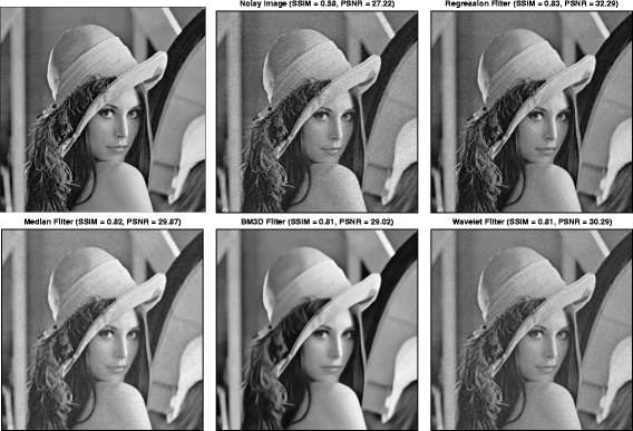
Applied Poisson noise. From left to right: a clean Lena, b noisy image, c denoised image using our L2 regression filter, d denoised image using median filter, e denoised image using BM3D, and f denoised image using wavelet filter
BM3D code is from https://github.com/glemaitre/BM3D
Matlab function ddencmp and wdencmp
Matlab function imnoise with option ’salt & pepper’
imageprocessingplace.com/root_files_V3/image_databases.htm
Matlab code P = U + σ×randn(size(U))
P=imnoise(U, ’poisson’); P=P+ σ×randn(size(U))

Abbreviations
- MSE:
-
Mean square error
- PSNR:
-
Peak signal-to-noise ratio
- SSIM:
-
Structural similarity
References
MR Adjout, F Boufares, in 2014 Tenth International Conference on Signal-Image Technology and Internet-Based Systems. A massively parallel processing for the multiple linear regression (IEEEMarrakech, 2014), pp. 666–671.
A Beck, M Teboulle, Fast gradient-based algorithms for constrained total variation image denoising and deblurring problems. IEEE Trans. Image Process. 18(11), 2419–2434 (2009).
J Bai, X Feng, Fractional-order anisotropic diffusion for image denoising. IEEE Trans. Image Process. 16(10), 2492–2502 (2007).
A Buades, B Coll, J-M Morel, Image denoising methods. A new nonlocal principle. SIAM Rev. 52(1), 113–147 (2010).
A Buades, B Coll, JM Morel, A review of image denoising algorithms, with a new one. Multiscale model. Simul. 4(2), 490–530 (2005).
H Burger, C Schuler, S Harmeling, in 2012 IEEE Conference on Computer Vision and Pattern Recognition (CVPR). Image denoising: can plain neural networks compete with bm3d? (IEEEProvidence, 2012), pp. 2392–2399.
P Chatterjee, P Milanfar, Patch-based near-optimal image denoising. IEEE Trans. Image Process. 21(4), 1635–1649 (2012).
K Dabov, A Foi, V Katkovnik, K Egiazarian, in Electronic Imaging 2006, International Society for Optics and Photonics. Image denoising with block-matching and 3d filtering (SPIE, the International Society for Optics and PhotonicsSan Jose, 2006).
K Dabov, A Foi, V Katkovnik, K Egiazarian, Image denoising by sparse 3-d transform-domain collaborative filtering. IEEE Trans. Image Process. 16(8), 2080–2095 (2007).
RA DeVore, B Jawerth, BJ Lucier, Image compression through wavelet transform coding. IEEE Trans. Inform. Theory. 38(2), 719–746 (1992).
DL Donoho, De-noising by soft-thresholding. IEEE Trans. Inform. Theory. 41(3), 613–627 (1995).
M Elad, M Aharon, Image denoising via sparse and redundant representations over learned dictionaries. IEEE Trans. Image Process. 15(12), 3736–3745 (2006).
R Eslami, H Radha, Translation-invariant contourlet transform and its application to image denoising. IEEE Trans. Image Process. 15(11), 3362–3374 (2006).
M Everingham, LV Gool, C Williams, J Winn, A Zisserman, The PASCAL Visual Object Classes Challenge 2012 (VOC2012) results. http://host.robots.ox.ac.uk/pascal/VOC/voc2012/index.html. Accessed 22 Mar 2018.
D Gabor, Information theory in electron microscopy. Lab. Investig. 14(6), 801–807 (1965).
G Ghimpeteanu, T Batard, M Bertalmio, S Levine, A decomposition framework for image denoising algorithms. IEEE Trans. Image Process. 25(1), 388–399 (2016).
S Gu, L Zhang, W Zuo, X Feng, in Proceedings of the IEEE Conference on Computer Vision and Pattern Recognition. Weighted nuclear norm minimization with application to image denoising (IEEEColumbus, 2014), pp. 2862–2869.
K Hirakawa, TW Parks, Image denoising using total least squares. IEEE Trans. Image Process.15(9), 2730–2742 (2006).
C Kervrann, J Boulanger, Optimal spatial adaptation for patch-based image denoising. IEEE Trans. Image Process. 15(10), 2866–2878 (2006).
A Levin, B Nadler, in IEEE Conference on Computer Vision and Pattern Recognition (CVPR). Natural image denoising: optimality and inherent bounds (IEEEBarcelona, 2011), pp. 2833–2840.
JS Lim, Two-dimensional signal and image processing (Prentice Hall, Englewood Cliffs, 1990).
M Lindenbaum, M Fischer, A Bruckstein, On gabor contribution to image enhancement. Pattern Recognit. 27:, 1–8 (1994).
H Liu, R Xiong, J Zhang, W Gao, in IEEE Conference on Computer Vision and Pattern Recognition. Image denoising via adaptive soft-thresholding based on non-local samples (IEEEBoston, 2015), pp. 484–492.
F Luisier, T Blu, M Unser, A new sure approach to image denoising: interscale orthonormal wavelet thresholding. IEEE Trans. Image Process. 16(3), 593–606 (2007).
F Luisier, T Blu, M Unser, Image denoising in mixed Poisson–Gaussian noise. IEEE Trans. Image Process. 20(3), 696–708 (2011).
J Mairal, F Bach, J Ponce, G Sapiro, A Zisserman, in 2009 IEEE 12th International Conference on Computer Vision. Non-local sparse models for image restoration (IEEEKyoto, 2009), pp. 2272–2279.
M Mäkitalo, A Foi, Optimal inversion of the Anscombe transformation in low-count poisson image denoising. IEEE Trans. Image Process. 20(1), 99–109 (2011).
X Mingxian, JJ Miller, EJ Wegman, Parallelizing multiple linear regression for speed and redundancy: an empirical study. J. Stat. Comput. Simul. 39(4), 205–214 (1991).
M Miller, N Kingsbury, Image denoising using derotated complex wavelet coefficients. IEEE Trans. Image Process. 17(9), 1500–1511 (2008).
M Mobasheri, S Zendehbad, Detection and elimination of striped noise in chris-proba sensor images. Symp. Adv. Sci. Technology-Commission-IV, 68–72 (2014).
S Parrilli, M Poderico, CV Angelino, L Verdoliva, A nonlocal SAR image denoising algorithm based on LLMMSE wavelet shrinkage. IEEE Trans. Geosci. Remote Sensing. 50(2), 606–616 (2012).
P Perona, J Malik, Scale space and edge detection using anisotropic diffusion. IEEE Trans. Patt. Anal. Mach. Intell. 12:, 629–639 (1990).
M Protter, M Elad, Image sequence denoising via sparse and redundant representations. IEEE Trans. Image Process. 18(1), 27–35 (2009).
T Tasdizen, in ICIP 15th IEEE International Conference on Image Processing. Principal components for non-local means image denoising (IEEESan Diego, 2008), pp. 1728–1731.
T Tasdizen, Principal neighborhood dictionaries for nonlocal means image denoising. IEEE Trans. Image Process. 18(12), 2649–2660 (2009).
J Wright, AY Yang, A Ganesh, SS Sastry, Y Ma, Robust face recognition via sparse representation. IEEE Trans. Pattern Anal. Mach. Intell. 31(2), 210–227 (2009).
Y Xie, S Gu, Y Liu, W Zuo, W Zhang, L Zhang, Weighted Schatten p-norm minimization for image denoising and background subtraction. IEEE Trans. Image Process. 25(10), 4842–4857 (2016).
R Yan, L Shao, Y Liu, Nonlocal hierarchical dictionary learning using wavelets for image denoising. IEEE Trans. Image Process. 22(12), 4689–4698 (2013).
L Yaroslavsky, M Eden, Fundamentals of digital optics (Birkhauser Boston, Boston, 1996).
L Yaroslavsky, in Proceedings of wavelet applications in signal and image processing IV. Local adaptive image restoration and enhancement with the use of dft and dct in a running window (SPIE, the International Society for Optics and PhotonicsDenver, 1996), pp. 1–13.
H Yu, L Zhao, H Wang, Image denoising using trivariate shrinkage filter in the wavelet domain and joint bilateral filter in the spatial domain. IEEE Trans. Image Process. 18(10), 2364–2369 (2009).
M Zhang, BK Gunturk, Multiresolution bilateral filtering for image denoising. IEEE Trans.Image Process. 17(12), 2324–2333 (2008).
H Zhang, J Yang, J Xie, J Qian, B Zhang, Weighted sparse coding regularized nonconvex matrix regression for robust face recognition. Inf. Sci. 394:, 1–17 (2017).
Acknowledgements
Not applicable.
Funding
This work is partly supported by NSF DMS-1228348 and ARO W911NF-17-1-0356.
Availability of data and materials
www.stat.purdue.edu/~xbw/JIVP/6SampleImages
It is the link for 6 sample clean images for displays.
www.stat.purdue.edu/~xbw/JIVP/100CleanImages
It is the link for 100 clean images in experiments.
Author information
Authors and Affiliations
Contributions
Both authors contribute to the original research in the paper. Both authors read and approved the final manuscript.
Corresponding author
Ethics declarations
Competing interests
The authors declare that they have no competing interests.
Publisher’s Note
Springer Nature remains neutral with regard to jurisdictional claims in published maps and institutional affiliations.
Rights and permissions
Open Access This article is distributed under the terms of the Creative Commons Attribution 4.0 International License (http://creativecommons.org/licenses/by/4.0/), which permits unrestricted use, distribution, and reproduction in any medium, provided you give appropriate credit to the original author(s) and the source, provide a link to the Creative Commons license, and indicate if changes were made.
About this article

Cite this article
Sharabati, W., Xi, B. A neighborhood regression approach for removing multiple types of noises. J Image Video Proc. 2018, 19 (2018). https://doi.org/10.1186/s13640-018-0259-9
Received:
Accepted:
Published:
DOI: https://doi.org/10.1186/s13640-018-0259-9