- Research
- Open access
- Published:
Line and circle detection using dense one-to-one Hough transforms on greyscale images
EURASIP Journal on Image and Video Processing volume 2016, Article number: 46 (2016)
Abstract
By estimating the first-order (direction) and second-order (curvature) derivatives in an image, the parameters of a line or circle passing through a point may be uniquely defined in most cases. This allows to compute a one-to-one Hough transform, every point in the image space voting for one unique point in the parameter space. Moreover, those parameters can be directly estimated on the greyscale image without the need to calculate the contour and without reducing the spatial support of the Hough transform, i.e. densely on the whole image. The general framework using multiscale derivatives is presented, and the one-to-one Hough dense transforms for detecting lines and circles are evaluated and compared with other variants of Hough transforms, from qualitative and computational points of view.
1 Introduction
The Hough transform (HT), one of the oldest algorithms of computer vision [1, 2], has been attracting a continuous interest for more than 50 years, as testified by a number of surveys [3–5], the most recent one [6], mentioning more than 2500 research papers, and citing around 100 post-2000 references. This is due not only to the constant development of applications based on graphics recognition but also to the elegance and generality of the Hough framework, allowing to detect analytical [7–10] as well as non-analytical [11–13] shapes in a wide variety of relevant manners.
The basic principle of the HT is to project the image data within a parameter space representing possible positions of a shape in the image space, then to search accumulation points in the parameter space, corresponding to the most probable positions of the shape in the image. Although many variations have been proposed until recently, it is remarkable that in most cases, the projection (voting process) is sparsely performed on contour or salient points of the image space. In addition, it is almost always performed using one of the two dual methods: one-to-many (one point in the image space votes for an multidimensional surface in the parameter space) or many-to-one (a set of points in the image space votes for one single point in the parameter space).
In this paper, we advocate the use of dense spatial derivatives instead of reducing the spatial support to a sparse set. Intuitively, this must make the vote more statistically significant and then have a positive influence on robustness. More unexpectedly, this should also lower the computational cost because it removes the selection process and, above all, because in the case of lines and circles, the voting is a one-to-one projection from the image to the parameter space. Although dense HTs have been proposed already, and one-to-one voting has also been used by some authors, to our knowledge, the two concepts have not been used together. Our contributions are the following: (1) a general framework for one-to-one dense Hough transform (DHT) using multiscale spatial derivatives, (2) practical algorithms based on this framework for line and circle detection and (3) a comparative study to evaluate the benefits and the weaknesses of the one-to-one DHTs.
To compare with other HTs, we define a computational protocol for evaluating the performance of line and circle detection algorithms. The algorithms are tested on real images with manually defined ground truth. Then, for every algorithm, we plot the number of true positive shapes as a function of the number of detected shapes. The robustness to noise and to illumination changes of the different algorithms and their variants are evaluated. We also compare the computational costs of the different methods.
This paper is organised as follows: Section 2 recalls the fundamentals for Hough transform and multiscale derivatives and present the related works. In Section 3, we present the one-to-one DHT for line and circle detection. Section 4 defines the evaluation protocol, presents comparative results of line and circle detection and discusses them. Section 5 finally outlines the contributions of this work and concludes.
2 Related works
2.1 Hough transform
An n-dimensional binary image I being a subset of \(\mathbb {R}^{n}\), an analytical shape may be defined by a parametric equation: \(\mathcal {C}^{\mathbf {a_{0}}} = \left \{\mathbf {x} \in \mathbb {R}^{n}; \phi (\mathbf {x},\mathbf {a_{0}}) = 0\right \}\), where x is the spatial variable, and \(\mathbf {a_{0}} \in \mathbb {R}^{m}\) is a constant parameter. Now for a specific \(\mathbf {x_{0}} \in \mathbb {R}^{n}\), the set \(\mathcal {D}^{\mathbf {x_{0}}} = \left \{\mathbf {a} \in \mathbb {R}^{m}; \phi (\mathbf {x_{0}},\mathbf {a}) = 0\right \}\), where a is the parametric variable, is a surface in the m-dimensional parameter space, which is the projection, or dual form of point x
0. The sum of all the projections of I is called the Hough transform of I relatively to ϕ:  where
where  is the indicator function of set A. The most representative shapes within I are finally detected by searching the maxima of \(\Gamma _{I}^{\phi }\).
For line detection, the polar parametric equation is preferred for uniform quantisation purposes [7]. The space variable is x=(x,y), the parametric variable is a=(θ,ρ) and the parametric equation is x cosθ+y sinθ=ρ. The dual form \(\mathcal {D}^{(x,y)}\) is a sine curve. For circle detection, the parametric variable is (c x ,c y ,r) and the parametric equation is (x−c x )2+(y−c y )2=r 2 [7]. The dual form \(\mathcal {D}^{(x,y)}\) is a conic surface.
In practice, both the image and the parameter space are quantised. The HT is classically applied on a binary image made of thin and regular curves, obtained using a contour detection algorithm. The transform is calculated using one of the two dual methods: (1) The one-to-many projection (a.k.a divergent transform), which consists in scanning every pixel x 0 of the binary image, and then incrementing \(\Gamma _{I}^{\phi }\) on the whole surface \(\mathcal {D}^{\mathbf {x_{0}}}\) as defined above. (2) The many-to-one projection (a.k.a convergent transform), which consists in considering every m-tuple of pixels {x i }1≤i≤m of the binary image such that there exists a unique a 0 in the parameter space such that for all x i , ϕ(x i ,a 0)=0 (e.g. m=2 for lines and m=3 for circles) and then increment only \(\Gamma _{I}^{\phi }(\mathbf {a_{0}})\).
One known drawback of the classical HT is their computational cost. If p is the number of voting pixels in the binary image, m the dimension of the parameter space, and k the average number of samples per dimension of the parameter space, the complexity of projection is proportional to pk m−1 for the one-to-many transform, and to \(\binom {p}{m}\) for the many to one. The most popular approaches to reduce the complexity consist in decreasing the number of voting pixels by randomly picking a subset of them. For the one-to-many transform, such approach is known as PHT, or probabilistic Hough transform [14–16]. In the case of many-to-one transforms, it is called RHT, or randomised Hough transform [17, 18]. Classic HT, PHT and RHT have been compared from qualitative and computational perspectives in [19] and [20].
Using the local derivatives to improve or to accelerate the HT has been done before, it was proposed for lines by O’Gorman and Clowes [21] and for differentiable curves by Shapiro [22]. In his review article, Maître [3] explicitly mentioned the one-to-one HT for lines and circles. However, these approaches have been scarcely used and—to our knowledge—only on binary curves, never directly on grey level images. The gradient information has been used in line detection for accelerating the HT [23] or for controlling the voting process to improve the progressive PHT [24]. Valenti and Gevers [25] have proposed an efficient eye centre location algorithm based on a voting scheme using the isophote curvature estimation. Recently, Yao and Yi [26] used the curvature of the contour to estimate the radius and then accelerate the circle HT. However, all these approaches still reduced the voting pixels to a thin contour previously calculated.
Kesidis and Papamarkos [27] have proposed an invertible grey level HT by using directly the grey level value of the pixels. In their circle detector, Atherton and Kerbyson [28] applied a collection of convolutions on the gradient image, which is equivalent to weighting the HT by the gradient. A dense vote using the gradient and without calculating the contours was performed for line detection by Dahyot [29]. But she used an estimated density kernel to spread the votes in the parameter space, resulting in a computational cost actually higher than the classical approach.
As a conclusion, amongst the few existing one-to-one HTs, none is a dense method, and none of the existing dense approaches is a one-to-one projection. The framework proposed in this paper, which combines the two, is a systematic approach based on (1) estimating the gradient and/or the curvature on the greyscale image, (2) performing, for all the pixels of the image space, a one-to-one vote in the parameter space, and (3) weighting the vote by the significance of the derivative measure. We argue that (i) generalising the vote to all the pixels make the DHT statistically more significant [29], (ii) the direct calculation on the grey level removes the dependence to the limits and parameters of the contour detection algorithm and, finally, (iii) although the number of voting points increases by one order of magnitude, the complexity is actually lower because the estimation of derivatives have a computational cost which is lower or comparable to the contour detection algorithm and the one-to-one voting process has a constant complexity. Let us now recall the useful bases on image derivatives.
2.2 Multiscale derivatives on greyscale images
When dealing with local structures in images, differential geometry is a very convenient framework and has been used for low-level image modelling and analysis for decades to perform contour detection [30], point tracking [31], optical flow estimation [32], corner [33], blob [34] or ridge detection [35]. From a biological point of view, the importance of local derivatives up to order two for the human visual system has been acknowledged a long time ago [36].
In the differential framework, the image I is considered as a differentiable function from \(\mathbb {R}^{2}\) to \(\mathbb {R}\). Let (O,x,y) be the Cartesian reference frame of \(\mathbb {R}^{2}\). We denote \(I_{x} = \frac {\partial I}{\partial x}\), \(I_{xx} = \frac {\partial ^{2} I}{\partial x^{2}}\) and so on.
At first order, if ∇I=(I x ,I y ) is the gradient vector, the value of the first derivative along any direction represented by unit vector v is given by
Thus, the derivative along the direction orthogonal to the gradient (isophote direction t) is zero, whereas the derivative in the gradient direction g is equal to the gradient magnitude \(||\nabla I|| = \sqrt {{I_{x}^{2}} + {I_{y}^{2}}}\). On every point p such that ||∇I(p)||>0, the gradient and isophote form a local reference frame (p,g,t) corresponding to first-order gauge coordinates (see Fig. 1). The isophote curve passing through p can be parameterised by the curvilinear coordinate s, such that

Gradient, isophote and curvature estimated at point P in a greyscale image
At second order, if \(H_{I} = \left (\begin {array}{ll} I_{xx} & I_{xy}\\ I_{xy} & I_{yy} \end {array}\right)\) is the Hessian matrix at point p, the value of the second derivative along any couples of direction represented by unit vectors u and v can be calculated by
One important second-order measure is the isophote curvature. Consider the displacement of a point along the isophote curve, where the curvilinear coordinate s is assimilated to time, and the local frame (p,g,t) corresponds to the Frenet frame. In this case, the isophote curvature can be defined as the radial acceleration \(\ddot {\mathbf {g}}(s)\), when the displacement is made at unit velocity, i.e. \(\dot {\mathbf {t}}(s) = 1\) (using the notation \(\dot {\mathbf {x}} = \frac {\partial \mathbf {x}}{\partial s}\) and \(\ddot {\mathbf {x}} = \frac {\partial ^{2} \mathbf {x}}{\partial s^{2}}\)).
Derivating Eq. 2 with respect to s provides
Since I t =0, if I g ≠0, we get \(\dot {\mathbf {g}} = 0\). Then, derivating again Eq. 4 with respect to s provides
Finally, since I t =0, \(\dot {\mathbf {t}} = 1\) and \(\dot {\mathbf {g}} = 0\) (if I g ≠0), we get
And by using Eqs. 1 and 3, we can get the expression of the isophote curvature κ in Cartesian coordinates [37]
The absolute value of the isophote curvature corresponds to the inverse of the radius of the osculating circle to the isophote curve (see Fig. 1), while its sign provides the polarity of the curvature (positive: brighter inside).
When I is a digital image, according to the scale space framework [36, 38, 39], the spatial derivatives are estimated relatively to a certain scale σ which represents the level of regularity, explicitely enforced by Gaussian smoothing
where ⋆ is the convolution and G σ the 2d Gaussian function of standard deviation σ (from now on, when working at a single scale, we will frequently omit the σ superscript).
In the next section, Hough transforms and multiscale derivatives are put together to form an effective framework for line and circle detection.
3 One-to-one dense Hough transforms
The one-to-one dense Hough transforms (DHT) for lines and circles are presented in this section. They are directly computed on greyscale images using spatial derivatives. The first-order derivatives (gradient vector) are used for the line detection, and the first- and second-order derivatives (gradient vector and Hessian matrix) are used for the circle detection. Section 3.1 exposes the general principles, then the algorithms are presented in Section 3.2. Section 3.3 discusses the implementation details and parameters, and Section 3.4 shows some results.
3.1 General principles
It can be deduced from Section 2.2 that at any image location p such that ||∇I(p)||≠0, the knowledge of the two first orders of spatial derivatives allows to calculate the equation of the line or circle possibly present at p. Furthermore, the scale space estimation of the derivative allows to effectively compute the line and/or circle present at many locations directly from the greyscale. This can be seen on Fig. 2, where the lines (a) and circles (b) passing through different locations in the image have been automatically computed using respectively the first-order and the two first-order derivatives. The basic principle of the one-to-one DHT is to generalise this computation to all pixels through a voting process.

Direct detection of lines and circles from partial derivatives. In the two images, the derivatives have been estimated at a few chosen locations (shown by the little red circles) from the grey levels using a scale estimation of σ=3.0. a Line deduced from the gradient direction (here, the segments with arrow represent the gradient vectors). b Circle deduced from the isophote curvature and the gradient direction: here, the segments with arrow have the direction of the gradient vector, their magnitude is the inverse of the absolute value of the isophote curvature, and their sense is the same as the gradient for the positive curvature (blue circles) and its opposite for the negative curvature (circles in cyan)
More explicitely, at the first order, using the classical (θ,ρ) polar parametrisation, where ρ is the distance between the line and the origin, and θ is the angle made by the normal to the line with the x axis, if there is a line passing through point p, we must have
i.e., θ p corresponds to the direction of the gradient vector and ρ p to the distance between the origin and the line passing through p and perpendicular to the gradient vector. To evaluate the significance of the location with respect to the presence of line, it is natural to use the strength of the first derivative, i.e., the magnitude of the gradient \(||\nabla I|| = \sqrt {{I_{x}^{2}} + {I_{y}^{2}}}\) (see Fig. 3 a, b).

Voting in one-to-one DHT (the estimation scale used here is σ=3.0; for visibility purposes, at most, one vote per 5×5 block is displayed). a Voting weight at order 1: the magnitude of the gradient. b Votes for the gradient direction (only votes with weights higher than 2.5 are displayed). c Voting weight at order 2: the Frobenius norm of the Hessian matrix. d Votes for the position of the centre of osculating circle (only votes with weights higher than 0.5 are displayed)
At the second order, using the (C,r) parametrisation, where \(C \in \mathbb {R}^{2}\) is the centre and r the radius of the circle, if there is a circle passing through point p, we must have
i.e., the radius r p is the inverse of the absolute curvature κ p calculated at point p using Eq. 7, and the centre C p is obtained by tracing from p the vector whose magnitude corresponds to the radius, whose direction is the same as the gradient and whose sense depends on the sign of curvature. Again, we can evaluate the significance of the location p with respect to the presence of circle by using the strength of the second derivative, i.e., the Frobenius norm of the Hessian matrix \(||H_{I}||_{F} = \sqrt {I_{xx}^{2} + 2I_{xy}^{2} + I_{yy}^{2}}\). The convergence of the most significant votes toward the potential circle centres is visible on Fig. 3 c, d.
In the multiscale DHT, we will combine the derivatives estimated at different scales. If the votes account for the relative importance of a given derivative at a certain location, it is advisable to normalise the corresponding derivative according to the scale and to the order of derivation σ [40]. Then, the multiscale voting weights will be σ||∇I|| at order 1 and σ 2||H I || F at order 2.
3.2 DHT algorithms
3.2.1 Line DHT
The one-to-one DHT algorithm for line detection using the (θ,ρ) parametrisation is presented on Table 1.
This algorithm is directly deduced from Eqs. 9 and 10. An example of 1-to-1 line DHT can be seen on Fig. 6 d.
3.2.2 Circle DHT basic (V1)
Table 2 shows the basic algorithm for circle detection, based on 1-to-1 dense votes in the 3d (c x ,c y ,ρ) parameter space.
This algorithm is directly deduced from Eqs. 11 and 12. An example of 1-to-1 circle DHT V1 can be seen on Fig. 8 (2, right).
3.2.3 Circle DHT two-pass (V2)
The straightforward implementation of the one-to-one DHT for circles does not provide good results in general. This is due to the fact that several scales of estimation are usually needed to improve the detection of the centres, but they also disperse the votes for the radius component, which makes the detection difficult.
To address this problem, a two-pass algorithm can be applied. The whole algorithm is detailed on Table 3. It first computes a one-to-one partial DHT Γ 1, where the parameter space is reduced to the 2d (c x ,c y ) centre space. This first pass (lines 3 to 13) then concentrates the votes for all radii, reducing the sparsity and improving the centre localisation. The N best centres are selected from Γ 1 (line 15), and then a second pass is applied to accumulate the possible radii for a circle centred on one of these N candidate centres. In this second pass (lines 17 to 27), one single scale (the smallest σ 1) is used, to determine for every pixel p, in a one-to-one manner, the centre and radius of a circle possibly passing through p (lines 18 to 21). Then, it is checked if the estimated centre matches one (or several) previously selected candidate centres, and when it does, the accumulator array Γ 2 for the corresponding candidate and radius is incremented (lines 22 to 26).
Two-pass algorithms are now classical in Hough-based circle detection [41–43], but their first pass is a one-to-many 2d HT, where the votes are made along straight lines, either defined by the gradient direction [41, 42], or by the bissector of a point pair chord [43]. In our V2 version, the first pass is a one-to-one DHT based on the isophote curvature. Figure 8 (4, right) shows an example of such first pass (centre detection).
3.3 Implementation and parameters
Although simpler in many aspects, the one-to-one dense Hough transform, like its one-to-many or many-to-one counterparts, is sensitive on implementation details and parameters. The purpose of this section is to go into deeper details on each part of the algorithms.
3.3.1 Weighting the votes
The DHT uses a norm-based censitary suffrage: all the pixels vote, but their vote is weighted according to the norm of the corresponding derivative. When using different scales, the scale should also take part to the weight as a scale space normalisation. The votes are then weighted by σ||∇I|| at order 1 and σ 2||H I || F at order 2. The justification of using this weight is that the relevant features (line or osculating circle positions) are poorly defined when the contrast (||∇I||) or the global curvature (κ) is too weak.
However, such weighting naturally favours the highly contrasted structures, which is not always desirable. A radical method for being contrast invariant is to use a true egalitarian suffrage, with uniform weight ω=1.0, which conversely may favour spurious structures like jpeg artefacts. Obviously, many trade-offs can be applied, like using a uniform weight but selecting the voting pixels with threshold or weighting by the logarithm of the norm. Different weighting strategies will be compared and discussed in the evaluation section (see Section 4).
3.3.2 Multiscale derivatives
A proper estimation of the derivatives is essential for the DHT. The poor results obtained using finite difference on curves, or small convolution kernels on greyscale images (particularly for the curvature), probably explain the very little attention received by one-to-one HT so far. Nevertheless, the scale space estimation of derivatives allows an accurate and noise robust estimation of gradient and curvatures at different scales. In this work, we used the recursive implementation of the (approximated) Gaussian convolution proposed by Young and van Vliet [44]. The best estimation scale locally depends on the image structure and the noise level. It could be selected automatically from the image [40], but simply aggregating the votes at the different scales with their different weights is actually faster and closer to the Hough spirit.
The number and the values of scales thus have an influence on the results. At larger scales, the number of structures decrease but their localisation is less precise: in the Hough space, the peaks are less numerous, but more flattened. In this sense, combining multiple scales can improve the detection, as illustrated on Fig. 4: the finer scales improve the localisation of the main peaks while the coarser scales reduce the influence of the spurious structures. Furthermore, the use of several scales may also improve the detection by reducing the sparsity of the DHT.

Influence of the multiscale: topographic close up around a maximum in the (θ,ρ) space for the 1-to-1 line DHT, using one single fine scale (a): σ=1.0, one single coarse scale (b): σ=4.0 and three scales (c): σ∈{1.0,2.0,4.0}
What was observed in our experiments (see Section 4) is that for line detection, the use of more than one scale is unnecessary for noise-free images. For circles, the V1 and V2 versions work better with multiple scales. For V2 version, the first pass uses several scales, as it clearly improves the detection of the centres, while the second pass (radius voting) performs better by using one single scale, the finest one. Figure 5 illustrates this behaviour by showing on a toy example that only the multiscale version of the V2 algorithm correctly detects all the circles.

Influence of the multiscale voting on the two-pass one-to-one DHT for circle detection. The image represents 15 black disks with radii ranging between 3 and 30 on a white background, with a Gaussian noise of 20%. Left: the original image with the 15 best circles overlaid in red. Right: the output of the first pass of the two-pass DHT (centre localisation)
3.3.3 Parameter space representation and maxima selection
The representation of the parameter space has a major influence on the precision of the detection and also on its complexity. The most classical method consists in quantising every dimension of the parameter space according to the desired precision of the detection, voting by simply incrementing the nearest node of the quantised space, and then choosing the highest local maxima as the best shapes. This is what is done for the one-to-many methods because a sufficiently high precision is needed to draw significant dual surfaces in the parameter space.
Because the comparative evaluation in the next section is performed against one-to-many methods, we have essentially used the same classical representation, referred to as “fine-grained parameter space”. This allowed to focus the comparison on the impact of our contribution, that is on the voting process, i.e., dense one-to-one vs. sparse one-to-many.
It is well known that detecting the N local maxima with highest value is not sufficient in general to avoid multiple detections (a beam of shapes corresponding to the same physical structure). In our experiments using fine-grained parameter space, we employed non-local maxima deletion as well as an exclusion distance criterion which consists in discarding, in the Hough space, all values whose distance to a previously selected point is below a certain threshold. Defining the exclusion ball in general should not be a fundamental problem, since it relates to the expected spatial distribution of the shapes.
The one-to-one, like the many-to-one transforms, are naturally sparser than the one-to-many transforms, every pixel voting for a single point. For circles, the sparsity of the basic one-to-one transform (V1) is still more important because of a larger parameter space. The sparsity can be moderated a priori by interpolating the votes and a posteriori by smoothing the transform. For the V1 version of the circle detector applied on Fig. 8 (2), a separable recursive exponential smoothing filter (γ=2.0) was applied in the 3d Hough space.
More interestingly, voting for one single location in the parameter space releases the strict need for quantisation. As done by Xu in the case of many-to-one RHT [17], dynamical accumulation data structures (e.g. lists or trees) can be used to store the estimated parameters without modifying them and then perform clustering-based accumulation search. The number of votes of the DHT being relatively high, and the dimension of the parameter space being low, one natural data structure is a simple grid like in the previous case, except that the step of the grid is much larger (it no longer depends on a desired localisation precision, but rather corresponds to the exclusion ball used to address multiple detections). The other difference is that instead of coding only a number of votes, every cell of the grid is a bucket containing a list of parameters with their associated weights.
In fact, the actual method used in our experiments is a very simple and efficient approximation of this large step bucket grid, calculated as follows: instead of storing the whole bucket list for every cell, we only keep one single weight value for every (large) cell, which finally makes the data structure identical as in the classical case, except that the quantification step is much larger (and then the resulting size much lower). However, to limit the effects of quantization, for every estimated parameter, the vote is multi-linearly interpolated over the corresponding cell bounds. For every pixel, let Q be the (real-valued) calculated parameter vector and ω Q the associated weight. Let ⌊Q⌋ be the integer valued vector made of the integer parts of every component of Q. Let R=Q−⌊Q⌋ the residual part of Q, with components in [0,1[. If m is the dimension of the parameter space, the interpolated vote consists in incrementing the 2m cells Γ(⌊Q⌋+B), for all B∈{0,1}m, by a value ω B such that:
Once the vote is completed, the best shapes are detected by searching the highest local maxima on the grid and then calculating the centroids of the parameters in the 3m neighbourhood for every selected maximum. This alternate method shall be referred to as “coarse-grained parameter space,” and its impact will be evaluated in Section 4.
3.4 DHT results
Figure 6 shows line detection results using the (θ,ρ) parameter space for the DHT (Fig. 6 d) compared with the classic exhaustive one-to-many HT (all the contour points are voting, Fig. 6 b). For the classic HT, the contour (Fig. 6 a) is obtained using Canny algorithm [45] with σ=1.5 and hysteresis threshold with t 1=1.0 and t 2=2.0. For the DHT, the transform is obtained by estimating the gradients at a single scale σ=1.5. For both methods, the parameter space was quantised using 720 samples for θ, the resolution for ρ being set according to the image diagonal, and the 50 best maxima were selected using the exclusion condition (θ e ,ρ e )=(15,12) (which means that two lines with parameters such that |θ 1−θ 2|<θ e AND |ρ 1−ρ 2|<ρ e cannot be detected at the same time, see Section 3.3). The 50 best lines are overlaid in magenta on the images that have been used for calculating the transform (Fig. 6 a, c).
Figure 7 shows two more results for line detection, with the same parameters as above. The 30 best lines are displayed for the first image, the 50 best ones for the second. These results are compared with the classic one-to-many HT calculated on contours (version called HoughStandard available on OpenCV with the same parameters as above).

Comparing the classic exhaustive one-to-many HT (a, b) and the one-to-one DHT (c, d) for line detection

Line detection, more results—left (lines in magenta): one-to-one DHT; right (lines in red): one-to-many HT (HoughStandard on OpenCV)
Figure 8 shows results for circle detection. Figure 8(1) corresponds to the classic one-to-many HT applied on the contour image. Figure 8(2) corresponds to the basic one-to-one DHT (our V1). Figure 8(3) shows the results for the two-pass 2–1 HT available in OpenCV [41], and Fig. 8(4) shows the results of the two-pass DHT (our V2). For the algorithms operating on contours (1 and 3), the Canny algorithm was applied with the same parameters as for the lines. For the dense algorithms (2 and 4), three scales were used for estimating the derivatives: σ∈{1.0,2.0,4.0}. Finally, for all algorithms, the radii were supposed bounded between 3 and 80, and to avoid multiple detections, an exclusion ball (C e ,r e )=((3,3),8) was applied (see Section 3.3). Figure 9 shows the results (40 best circles) on two other images for the two two-pass algorithms (same parameters).

Comparing different algorithms for circle detection. The 40 best circles are displayed. (1) and (3) operate on the contours, (2) and (4) on the grey level. For (1) and (2), one single plane from the 3d transform is shown (plane of equation r=25). For (3) and (4) is shown the 2d transform corresponding to the output of the first pass (centre localisation)

Circle detection, more results—left (circles in yellow): one-to-one two-pass DHT; right (circles in red): two-pass 2–1 HT (OpenCV)
4 Qualitative evaluation
This section is dedicated to the qualitative evaluation of the DHT for line and circle detection. First, the evaluation protocol is presented and the proposed metrics are justified. Then, we apply this evaluation, first to line detection, and then to the two versions of circle detection. The DHT algorithms are qualitatively compared with classic and state-of-the art HT algorithms available on the OpenCV library [16, 41, 46] and also with other state-of-the art line and circle detectors based on the HT, such as the randomised Hough transform [17] and the curvature aided circle detector [26].
4.1 Evaluation protocol and metrics
Line and circle detection algorithms are usually evaluated using synthetic binary images, showing different configurations of size/length, orientation, occlusion or noise, depending on the properties that need to be assessed. For obvious reasons, the DHTs need to be evaluated on greyscale images. The following protocol was applied:
-
One natural greyscale image showing significant amount of lines (resp. circles) was chosen, and its “ground truth” was manually set.
-
Every algorithm is assessed according to the proportion of ground truth lines (resp. circles) it detects, as a function of number of selected maxima.
-
To evaluate the sensitivity of the algorithms, the same measure is performed on images with three kinds of distortion: (1) additive noise, (2) impulse noise and (3) non-uniform illumination.
4.1.1 Voronoi-based detection rate
Our evaluation metrics is based on a matching criterion, using a distance in the parameter space. The ground truth image defines a set of ground truth points in the parameter space. The Voronoi tessellation [47] associated to this point cloud allows to match every detected curve to its most likely ground truth. If the distance to the matched ground truth is less than a determined threshold, then the corresponding curve is considered detected; otherwise, it is a “false” detection. Obviously, only the closest true detection is counted for each ground truth curve. Figure 10 shows the application of this principle for line detection on the House image.

Ground truth and matching principles. a Ground truth curves superimposed (in blue) on the image. b Corresponding point cloud in the parameter space with its Voronoi tessellation. The line {θ=0} is represented to mark the extension of the diagram to negative values of θ. c Detected curves (in red). d Matching the candidate curves in Hough space
Regarding lines, some precautions must be taken when using the Euclidean distance in the classic (θ,ρ) space because some discontinuities may appear when ρ is close to zero, the lines (θ,ρ) and (π−θ,ρ) being in that case close in the image space, but not in the parameter space. To address this problem, the (θ,ρ) space is extended to negative values of ρ, every ground truth line (θ,ρ) being duplicated to its equivalent (π−θ,−ρ), at least for the small values of ρ. The matching is then performed in this extended Voronoi diagram.
A wrong detection may be due to a false alarm (a curve absent from the ground truth) or to multiple detections of a right curve. The manual ground truth collection being largely subjective, measuring the false alarm rate did not turn out relevant. The wrong detections being—at least for clean images— essentially due to multiple detections, the quality of detection depends much on the quantisation of the parameter space and the maxima selection procedure. As the main contribution of this work is independent of these steps, the different HTs were compared using the same parameter space and selection steps.
Finally, the evaluation metrics we chose is the recall, i.e. the rate of ground truth curves that have been detected, as a function of the number of detected lines which is simply the number of selected maxima, the HT being actually a localisation, and not a detection algorithm.
4.1.2 Image distortions
To assess the sensitivity of the different algorithms and to better understand the importance of their parameters, the evaluation has been performed on distorted images. The first considered distortion is additive noise: different amounts of Gaussian noise have been added to the input images before performing the detection. The noise level is measured by the signal to noise ratio (SNR). The second one is impulse (i.e. salt and pepper) noise, whose intensity is measured as the proportion p of pixels set to aberrant values. The third one is non uniform illumination: let c be a non-uniformity factor. The distorted image is obtained by multiplying every greyscale I(x,y) by the horizontal ramp defined by \(r(x) = \frac {w}{cx+w}\), where w is the width of the image.
4.2 Line detection
We evaluated the DHT for line detection using the previous protocol on the House image with its ground truth (see Fig. 10). First, we performed a parametric study of the algorithm on different conditions. The results can be seen on Fig. 11 and can be interpreted as follows:
-
One single small scale (i.e. 1≤σ≤2) is generally sufficient for noise-free images, and sometimes better, since larger scales may fuse close lines or miss some segments.
Fig. 11 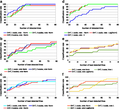
Parametric study of the DHT for line detection. a Influence of the number of scales (NS) on clean image. b Influence of the voting strategy (VS) on clean image. c, d Influence of NS and VS on noisy image (SNR = 5). e, f Influence of NS and VS on non-uniform contrast image (c=4)
-
Using two of three scales slightly improve the results for noisy images.
-
Regarding the weighting policy, the use of ||∇I|| or log(||∇I||) works equally well in the different conditions, and much better than using uniform weights, except for non-uniform illumination, when the number of detected lines becomes high.

Figure 12 shows the evaluation curves and Fig. 13 the corresponding detection results of the DHT, compared with other algorithms: (1) the standard one-to-many exhaustive HT (SHT), (2) the state-of-the-art progressive probabilistic HT (PPHT) [16] available from OpenCV and (3) the randomised HT (RHT) [17]. The three competitor algorithms are computed on the contour image obtained using Canny’s algorithm [45]. Algorithm 1 is the standard one-to-many approach, where all the contour pixels vote for a complete sine curve on the discrete parameter space, with a uniform vote. Algorithm 2 is also a one-to-many approach, except that only a fraction of the contour pixels are randomly chosen, with dynamic mechanisms to adapt the parameters to the lengths of significant lines. Finally, Algorithm 3 is a randomised many-to one approach, which randomly picks couples of points from the contour image, and then votes for the unique corresponding point in the parameter space.

Comparison between the DHT and others HT for line detection. a On clean image. b On image with additive noise (SNR = 5). c On image with salt and pepper noise (p=5%). d On non-uniform contrast image (c=4). Each colour corresponds to a different method. Red DHT, green RHT, blue SHT, magenta PPHT

50 best detected lines of the different algorithms in different conditions. Row 1: The SHT uses exhaustive one-to-many voting on Canny contour image (parameters of the Canny detector are σ=1, t 1=6, t 2=1 for column 1, σ=2, t 1=6, t 2=5 for column 2 and σ=1, t 1=3, t 2=1 for column 3). Row 2: the DHT (our method) uses dense voting weighted with the gradient norm, and three scales of estimation (same parameters for the three conditions). Row 3: the PPHT uses one-to-many scheme and adaptive random voting on Canny contour image. (Canny’s parameters vary like row 1; the threshold for line decision is 50 for column 1, 20 for column 2 and 10 for column 3). Row 4: the RHT uses many-to-one random voting scheme on Canny contour image. (Canny’s parameters vary like row 1)
4.3 Circle detection
The DHT was evaluated the same way for circle detection, using the radar ahead image as ground truth (Fig. 14). From the parametric study (Fig. 15), the following remarks can be made:
-
The two-phase version (V2) works much better than the direct (V1) version in all cases.
-
Unlike the lines, the use of two or three scales significantly improves the results, even for clean images.
-
Using the Frobenius norm of the Hessian matrix (without multiplying by the squared sigma) seems the best weighting policy, except for the non-uniform contrast images, where the constant weight seems the least bad option.
-
The method is pretty insensitive to noise; on the contrary, the results dramatically drops when the contrast turns non-uniform.

Test image for circle detection with ground truth (20 circles drawn in pink)

Parametric study of the DHT for circle detection. a Influence of the number of scales (NS) on clean image. b Influence of the voting strategy (VS) on clean image. c, d Influence of NS and VS on noisy image (SNR = 5). e, f Influence of NS and VS on non uniform contrast image (c=4)
The V2 DHT for circle detection was also compared to the following algorithms: (1) The classic one-to-many HT (SHT) computed on Canny’s contour (every pixel of the contour vote for a whole conic surface in the 3d parameter space). (2) The 2–1 HT for circle detection from OpenCV [41]. This algorithm is a two-pass one-to-many method, computed on a contour image also, which estimates in the first pass the gradient direction for every voting pixel, then votes on the straight line orthogonal to this direction, in the 2d parameter space restricted to the centre (c x ,c y ). The second pass looks for the best radius for a selection of the best centres, in the same manner as the V2 DHT. (3) The randomised HT (RHT), a many-to-one approach [17], which randomly picks point triplets from a contour image and then vote for a unique point in the parameter space. (4) The curvature aided circle detector (CACD), which estimates the curvature on the contour image [26] to perform a one-to-one vote using accumulation arrays of different radius ranges. The charts and the corresponding result images of this comparative evaluation may be seen on Figs. 16 and 17.

Comparison between the DHT and the other HTs for circle detection. a On clean image. b On image with additive noise (SNR = 5). c On image with salt-and-pepper noise (p=5%). d On non-uniform contrast image (c=4). Each colour corresponds to a different method. Red DHT, green RHT, blue SHT, magenta 2–1 HT, yellow CACD

50 best circles of the different algorithms in different conditions. Row 1: the SHT uses exhaustive one-to-many voting on Canny contour image (parameters of the Canny detector are σ=2, t 1=6, t 2=3 for column 1, σ=2, t 1=6, t 2=4 for column 2 and σ=1.5, t 1=2, t 2=1 for column 3). Row 2: the DHT V2 (two-pass) uses three scales of estimation, and dense voting weighted with Frobenius norm of the Hessian for columns 1 and 2, and uses two scales and uniform weight for column 3. Row 3: the 2–1 HT from OpenCV uses two-pass voting on Canny contour image. Row 4: the RHT uses many-to-one voting on Canny contour image. Row 5: the CACD uses one-to-one voting on Canny contour image. (For those three last methods, Canny’s parameters vary like the method of row 1)
4.4 Maxima selection and computational considerations
Finally, the influence of the parameter space representation, namely, “fine grained quantisation” vs. “coarse grained quantisation” with interpolated votes and centroid selection was evaluated. See Fig. 18: it can be seen here that the results with the coarse grained strategy are just slightly worse, although they are much more computationally efficient.

Influence on the DHT of representing the parameter space using classic “fine grained quantisation” of the parameter space or “coarse grained quantisation” with interpolated votes and centroid selection. a For line detection, b for circle detection
Regarding computational efficiency, Table 4 outlines the general complexity figures of the different HT versions that have been presented in this paper. To account for the different variants and optimisations, the results are presented in a proportional manner (\(\mathcal {O}(x)\) means that the number of operations is proportional to parameter x). In the table, every row corresponds to a different category of HT algorithm, every column to a different step of the algorithm. The different parameters appearing in the table are explained as follows:
-
n is the geometric mean number of samples per dimension in the image space (n 2 is the number of pixels).
-
p is the number of binary contour pixels.
-
m is the dimension of the parameter space.
-
k is the geometric mean number of samples per dimension in the (fine grained) parameter space (k m is the number of parameter voxels).
-
z is the geometric mean number of samples per dimension in the exclusion ball.
-
s is the number of scales used in the DHT.
For the computation of contours, the \(\mathcal {O}(n^{2})\) factor comes from the local estimation of the derivatives and the \(\mathcal {O}(p)\) factor comes from the hysteresis threshold applied to the gradient norm. For the DHT, the estimation of the derivatives has the same complexity as the first part of contour detection, but has to be multiplied by the number of scales. It is recalled that one single scale is currently used for lines and no more than two or three for circles. For the Hough transform itself (voting process), the one-to-many factor k m−1 comes from the dimension of the dual shape, and for many-to-one methods, the \(\binom {p}{m}\) factor comes from the combinatorial choices of m points amongst p contour points. The classical ways to lower the complexity is to decrease the multiplying coefficient to this factor by picking only a fraction of the contour points (one-to-many PHT) or of the choices of m points (many-to-one RHT). For the DHT, the cost of voting is obviously constant. This means that globally, the cost of the DHT is of the same order or lower than the contour detection, which is only the pre-processing step of the classic HT. For the last step, namely the maxima extraction from the parameter accumulator, the complexity is typically higher for one-to-many methods where a higher resolution of the parameter space is needed, than for many-to-one or one-to-one methods, where no quantification is strictly needed, or where a coarser resolution associated with interpolation mechanisms can be used.
As a complement to these theoretical considerations, we also compared in Table 5 the actual computation time between the different methods: our proposed method (DHT), randomized Hough transform (RHT) [17], standard Hough transform (SHT) [1], progressive probability Hough transform (PPHT) [16], curvature aided Hough transform (CACD) [26] and 2–1HT [41]. Note that DHT, SHT and RHT are applicable for both line and circle detection. Those figures only measure the computation of the Hough transform, not the maxima selection, in order to focus on our contribution. They have to be interpreted carefully, since the experiments were all made on the same hardware platform (a CPU Intel Duo cores, 2.6 GHz with RAM 3Gb), but using different software implementations, including distinct languages and different levels of optimisation. We use the images of Fig. 10 (512 × 512 pixels) and Fig. 14 (277 × 492 pixels), respectively, for line and circle detection. The default parameters of OpenCV or the parameters recommended by the authors were used. For the RHT method, we followed the suggestion of the authors of setting the number of point tuples (i.e. pairs or triplets) picked from the contours, equal to the number of pixels of the considered image. Obviously, the computation time of the exhaustive SHT is considerable. The RHT, PPHT and 2–1 HT approaches reduce significantly the computation time by drastically decreasing the number of votes. Finally, our DHT approach is also very computationnally efficient by removing the segmentation (contour) step and performing a one-to-one vote.1
5 Conclusions
We have presented in this paper a unified framework for computing dense Hough transforms directly from the greyscale images, without reducing the support to contour or interest points. By being independent on the quality of the contours or any other pre-processing step, the voting process is less sensitive to image perturbations. By allowing all the pixels to vote, it is more statistically significant. The weight of the vote can be softly adjusted by using the significance of the contrast or the curvature, provided by the gradient magnitude or the Frobenius norm of the Hessian matrix.
Another fundamental advantage of the DHT for detecting lines or circles is the unique determination of the parameter from the spatial derivatives, which allows to perform a one-to-one voting process, thus improving dramatically the global efficiency of the Hough transform.
We have proposed a multiscale voting procedure that allows: (1) to improve the noise robustness and (2) to enhance the detection of circles within a wide range of radii, by simply suming scale-normalised votes over the different scales.
We have proposed an evaluation protocol to assess the results of line and circle detection algorithms on natural grey level images and applied this evaluation on the DHT, first to provide a parametric study of these algorithms and then to compare them to other classic and state-of-the-art versions of line and circle detectors based on Hough transforms. We have shown that the qualitative results obtained by the DHT are of the same level than the other HT, while being less sensitive to image perturbations, and more computationally efficient.
In our future works, we are going to produce optimised versions of the one-to-one DHT for line and circle detections, in order to better promote and spread their use in the community. We are also working on generalised DHT [48] to extend the advantages of these algorithms to object detection, tracking and recognition [49, 50].
6 Endnote
1 These methods were implemented using different programming frameworks and languages: dense HT: C++, RHT: Matlab, SHT: Matlab, CACD: Matlab, PPHT: OpenCV/C++, 2–1HT: OpenCV/C++.
References
PVC Hough, in Int. Conf. High Energy Accelerators and Instrumentation. Machine analysis of bubble chamber pictures, (1959), pp. 554–556, http://inspirehep.net/record/919922?ln=en.
A Rosenfeld, Picture processing by computer. ACM Comput. Surv.1(3), 147–176 (1969). doi:10.1145/356551.356554.
H Maître, Un panorama de la transformation de Hough. Traitement du Signal. 2(4), 305–317 (1985).
J Illingworth, J Kittler, A survey of the Hough transform. Comput. Vis. Graph. Image Process.44(1), 87–116 (1988). doi:10.1016/S0734-189X(88)80033-1.
VF Leavers, Which Hough transform?CVGIP: Image Underst.58(2), 250–264 (1993). doi:10.1006/ciun.1993.1041.
P Mukhopadhyay, BB Chaudhuri, A survey of Hough transform. Pattern Recognit.48(3), 993–1010 (2015). doi:10.1016/j.patcog.2014.08.027.
RO Duda, PE Hart, Use of the Hough transformation to detect lines and curves in pictures. Commun. ACM. 15(1), 11–15 (1972). doi:10.1145/361237.361242.
N Bennett, R Burridge, N Salto, A method to detect and characterize ellipses using the Hough transform. IEEE Trans. Pattern Anal. Mach. Intell.21(7), 652–657 (1999). doi:10.1109/34.777377.
J Song, MR Lyu, A Hough transform based line recognition method utilizing both parameter space and image space. Pattern Recognit.38(4), 539–552 (2005). doi:10.1016/j.patcog.2004.09.003.
D Walsh, AE Raftery, Accurate and efficient curve detection in images: the importance sampling Hough transform. Pattern Recognit.35(7), 1421–1431 (2002). doi:10.1016/S0031-3203(01)00114-5.
DH Ballard, Generalizing the Hough transform to detect arbitrary shapes. Pattern Recognit.13(2), 111–122 (1981). doi:10.1016/0031-3203(81)90009-1.
B Leibe, A Leonardis, B Schiele, in Toward Category-Level Object Recognition. Lecture Notes in Computer Science, vol. 4170. An implicit shape model for combined object categorization and segmentation (SpringerSiracusa, Italy, 2006), pp. 508–524, doi:10.1007/11957959-26.
V Ferrari, F Jurie, C Schmid, From images to shape models for object detection. Int. J. Comput. Vis.87(3), 284–303 (2010). doi:10.1007/s11263-009-0270-9.
RS Stephens, Probabilistic approach to the Hough transform. Image Vis. Comput.9(1), 66–71 (1991). doi:10.1016/0262-8856(91)90051-P.
N Kiryati, Y Eldar, AM Bruckstein, A probabilistic Hough transform. Pattern Recognit.24(4), 303–316 (1991). doi:10.1016/0031-3203(91)90073-E.
J Matas, C Galambos, JV Kittler, Robust detection of lines using the progressive probabilistic Hough transform. Comput. Vis. Image Underst.78(1), 119–137 (2000). doi:10.1006/cviu.1999.0831.
L Xu, E Oja, P Kultanen, A new curve detection method: randomized Hough transform (RHT). Pattern Recognit. Lett.11(5), 331–338 (1990). doi:10.1016/0167-8655(90)90042-Z.
L Xu, A unified perspective and new results on RHT computing, mixture based learning, and multi-learner based problem solving. Pattern Recognit.40(8), 2129–2153 (2007). doi:10.1016/j.patcog.2006.12.016.
H Kälviäinen, P Hirvonen, L Xu, E Oja, Probabilistic and non-probabilistic Hough transforms: overview and comparisons. Image Vis. Comput.13(4), 239–252 (1995). doi:10.1016/0262-8856(95)99713-B.
N Kiryati, H Kälviäinen, S Alaoutinen, Randomized or probabilistic Hough transform: unified performance evaluation. Pattern Recognit. Lett.21(13-14), 1157–1164 (2000). doi:10.1016/S0167-8655(00)00077-5.
F O’Gorman, MB Clowes, Finding picture edges through collinearity of feature points. IEEE Trans. Comput.C-25(4), 449–456 (1976). doi:10.1109/TC.1976.1674627.
SD Shapiro, Feature space transforms for curve detection. Pattern Recognit.10(3), 129–143 (1978). doi:10.1016/0031-3203(78)90022-5.
SM Karabernou, F Terranti, Real-time FPGA implementation of Hough transform using gradient and CORDIC algorithm. Image Vis. Comput.23(11), 1009–1017 (2005). doi:10.1016/j.imavis.2005.07.004.
C Galambos, J Kittler, J Matas, Gradient based progressive probabilistic Hough transform. Vis. Image Signal Process. IEE Proc.148(3), 158–165 (2001). doi:10.1049/ip-vis:20010354.
R Valenti, T Gevers, in IEEE Conference on Computer Vision and Pattern Recognition (CVPR’08). Accurate eye center location and tracking using isophote curvature, (2008), pp. 1–8, doi:10.1109/CVPR.2008.4587529.
Z Yao, W Yi, Curvature aided hough transform for circle detection. Expert Syst. Appl.51:, 26–33 (2016). doi:10.1016/j.eswa.2015.12.019.
AL Kesidis, N Papamarkos, On the gray-scale inverse Hough transform. Image Vis. Comput.18(8), 607–618 (2000). doi:10.1016/S0262-8856(99)00067-0.
TJ Atherton, DJ Kerbyson, Size invariant circle detection. Image Vis. Comput.17(11), 795–803 (1999). doi:10.1016/S0262-8856(98)00160-7.
R Dahyot, Statistical Hough transform. IEEE Trans. Pattern Anal. Mach. Intell.31(8), 1502–1509 (2009). doi:10.1109/TPAMI.2008.288.
D Marr, E Hildreth, Theory of edge detection. Proc. R. Soc. London B: Biol. Sci.207(1167), 187–217 (1980). doi:10.1098/rspb.1980.0020.
C Tomasi, J Shi, in Proc. IEEE Conf. on Comp. Vision and Patt. Recog. Good features to track, (1994), pp. 593–600, doi:10.1109/CVPR.1994.323794.
BKP Horn, BG Schunck, Determining optical flow. Technical report (Massachusetts Institute of Technology, Cambridge, MA, USA, 1980).
C Harris, M Stephens, in Proceedings of the 4th Alvey Vision Conference. A combined corner and edge detector, (1988), pp. 147–151, http://citeseer.ist.psu.edu/viewdoc/summary?doi=10.1.1.231.1604.
DG Lowe, Distinctive image features from scale-invariant keypoints. Int. J. Comput. Vis.60(2), 91–110 (2004). doi:10.1023/B:VISI.0000029664.99615.94.
T Lindeberg, Edge detection and ridge detection with automatic scale selection. Int. J. Comput. Vis.30(2), 117–156 (1998). doi:10.1023/A:1008097225773.
J Koenderink, The structure of images. Biol. Cybernet.50(5), 363–370 (1984). doi:10.1007/BF00336961.
BMT Haar Romeny, Front-end vision and multi-scale image analysis. Computational Imaging and Vision (Kluwer Academic Publishers, Dordrecht, Boston, London, 2003).
AP Witkin, in Proceedings of the Eighth International Joint Conference on Artificial Intelligence - Volume 2. IJCAI’83. Scale-space filtering (Morgan Kaufmann Publishers Inc.Karlsruhe, West Germany, 1983), pp. 1019–1022.
L Florack, B Ter Haar Romeny, M Viergever, J Koenderink, The Gaussian scale-space paradigm and the multiscale local jet. Int. J. Comput. Vis.18(1), 61–75 (1996). doi:10.1007/BF00126140.
T Lindeberg, Feature detection with automatic scale selection. Int. J. Comput. Vis.30(2), 79–116 (1998). doi:10.1023/A:1008045108935.
HK Yuen, J Princen, J Illingworth, J Kittler, Comparative study of Hough transform methods for circle finding. Image Vis. Comput.8(1), 71–77 (1990). doi:10.1016/0262-8856(90)90059-E.
R Chan, New parallel Hough transform for circles. Comput. Digital Techniques, IEE Proc.138(5), 335–344 (1991).
D Ioannou, W Huda, AF Laine, Circle recognition through a 2d Hough transform and radius histogramming. Image Vis. Comput.17(1), 15–26 (1999). doi:10.1016/S0262-8856(98)00090-0.
IT Young, LJ van Vliet, Recursive implementation of the Gaussian filter. Signal Process.44(2), 139–151 (1995). doi:10.1016/0165-1684(95)00020-E.
J Canny, A computational approach to edge detection. IEEE Trans. Pattern Anal. Mach. Intell.8(6), 679–698 (1986). doi:10.1109/tpami.1986.4767851.
C Kimme, D Ballard, J Sklansky, Finding circles by an array of accumulators. Commun. ACM. 18(2), 120–122 (1975). doi:10.1145/360666.360677.
S Fortune, in Proceedings of the Second Annual Symposium on Computational Geometry. SCG ’86. A sweepline algorithm for Voronoi diagrams (ACMYorktown Heights, NY, USA, 1986), pp. 313–322, doi:10.1145/10515.10549.
A Manzanera, in Proceedings of the Sixth International Workshop on Medical and Healthcare applications(AMINA’12). Dense Hough transforms on gray level images using multi-scale derivatives (invited conference) (MahdiaTunisia, 2012), pp. 55–62.
J Gall, A Yao, N Razavi, L Van Gool, V Lempitsky, Hough forests for object detection, tracking, and action recognition. IEEE Trans. Pattern Anal. Mach. Intell.33(11), 2188–2202 (2011). doi:10.1109/TPAMI.2011.70.
O Barinova, VS Lempitsky, P Kohli, On detection of multiple object instances using hough transforms. IEEE Trans. Pattern Anal. Mach. Intell.34(9), 1773–1784 (2012). doi:10.1109/CVPR.2010.5539905.
Acknowledgements
We gratefully acknowledge the financial contribution of research cluster DIGITEO through the funding of Phuong Nguyen’s post-doctoral position.
Authors’ contributions
AM designed the one-to-one multiscale dense Hough transform framework and performed the first implementation. He wrote the sections dedicated to related works and theoretical contributions. XX designed the initial evaluation protocol and performed the first evaluations. TPN improved the evaluation protocol and the dense Hough transform implementation. He conducted all the comparative evaluation experiments and wrote the sections dedicated to the results and the discussion. All authors read and approved the manuscript.
Competing interests
The authors declare that they have no competing interests.
Author information
Authors and Affiliations
Corresponding author
Rights and permissions
Open Access This article is distributed under the terms of the Creative Commons Attribution 4.0 International License (http://creativecommons.org/licenses/by/4.0/), which permits unrestricted use, distribution, and reproduction in any medium, provided you give appropriate credit to the original author(s) and the source, provide a link to the Creative Commons license, and indicate if changes were made.
About this article

Cite this article
Manzanera, A., Nguyen, T. & Xu, X. Line and circle detection using dense one-to-one Hough transforms on greyscale images. J Image Video Proc. 2016, 46 (2016). https://doi.org/10.1186/s13640-016-0149-y
Received:
Accepted:
Published:
DOI: https://doi.org/10.1186/s13640-016-0149-y