- Research
- Open access
- Published:
Integrating clustering with level set method for piecewise constant Mumford-Shah model
EURASIP Journal on Image and Video Processing volume 2014, Article number: 1 (2014)
Abstract
In the paper, we present an efficient method to solve the piecewise constant Mumford-Shah (M-S) model for two-phase image segmentation within the level set framework. A clustering algorithm is used to find approximately the intensity means of foreground and background in the image, and so the M-S functional is reduced to the functional of a single variable (level set function), which avoids using complicated alternating optimization to minimize the reduced M-S functional. Experimental results demonstrated some advantages of the proposed method over the well-known Chan-Vese method using alternating optimization, such as robustness to the locations of initial contour and the high computation efficiency.
1 Introduction
Image segmentation is one of the most important and critical tasks towards high-level vision modelling and analysis. The segmentation problem can be formulated as follows: given an image I ∈ L2(Ω) on a two-dimensional domain Ω (assumed to be bounded, smooth, and open), one seeks out a closed ‘edge set’ C and all the connected components Ω1,…, Ω k of Ω\C so that by certain suitable visual measure, the image I is discontinuous along C while smooth or homogeneous on each segment Ω i (i = 1,…, k). Until now, a wide variety of techniques including variational methods [1, 2] have been proposed for image segmentation.
Variational methods for image segmentation have had great success, which are characterized by deriving an energy functional from some a priori mathematical model and minimizing this energy functional over all possible partitions. Among them, the Mumford-Shah (M-S) model [3] is one of the most widely studied mathematical models for image analysis. The M-S functional contains a data fidelity term and two/a regularity terms imposing a piecewise smooth/constant representation of an image and penalizing the Hausdorff measure of the set of discontinuities, resulting in simultaneous restoration and segmentation. Minimizing the M-S functional involves determining both a function and a contour across which smoothness is not.
The M-S functional has been extensively used in image segmentation [4–7]; however, the numerical method for solving the model is difficult to implement when direct implementations are performed. Therefore, in practice, one of the major challenges is to develop efficient algorithms to compute high-quality minimizes of this functional.
One of the earliest attempts is based on so-called continuation methods, such as simulated annealing [8] and the graduated non-convexity procedure [9]. The idea is to minimize the original energy by gradually decreasing a continuation parameter. However, the performances of these methods largely depend on the dynamics of the continuation parameter and therefore tend to get stuck in bad local minima.
Based on the level set method [10, 11], a very successful method is first introduced by Chan and Vese [12, 13] to solve the piecewise constant M-S model. After the Chan and Vese's work, different models based on the M-S functional with level set methods have been developed and widely adopted in various image applications [14–17].
Chan and Vese [12] primarily solve a special case of the M-S model where the binary case of two regions was considered and develop the widely used ‘active contours without edges’ model. For piecewise constant M-S model, Shen [18] uses gamma convergence formulation to the piecewise constant M-S model; it can be regarded as a diffuse interface method in which the ‘edges’ in the segmentation are represented as thin transition layers, and implementation is completed by the iterated integration of a linear Poisson equation. Esedoĝlu and Tsai [19] propose a very efficient minimization method based on the threshold dynamics, by alternating the solution of a linear parabolic partial differential equation and simple thresholding. In [20], Bresson et al. propose a global minimization of the active contour model based on the piecewise constant M-S model, in which the dual formulation is to be applied in minimization of the model and present a fast algorithm. These methods allow to compute high-quality solutions of the piecewise constant M-S functional. However, these methods solving the M-S functional involve alternating optimization [21, 22] of the reconstruction function and the contour.
In this paper, following the Chan-Vese (C-V) method, we propose an efficient method for minimizing the piecewise constant M-S functional. Unlike the existing methods above, our method to minimize the M-S functional avoids the use of complicated alternating optimization.
The remainder of this paper is organized as follows. In Section 2, we describe the M-S model, the C-V method and c-means clustering algorithm. Section 3 presents the proposed method. In Section 4, the proposed method is validated by some experiments on synthetic and real images. This paper is summarized in Section 5.
2 Related works
2.1 The M-S model
The M-S model [3] is a variational problem for approximating an image by a piecewise smooth image of minimal complexity. Let I: Ω ⊂ ℝ × ℝ → ℝ be a given image, the M-S functional is defined as
where u is a piecewise smooth approximation to the image I, μ and v are two positive constants to balance the terms; and C is the union of a finite number of curves, |C| is the length of C, and Ω\C is the domain excluding the curve C.
The solution image obtained by minimizing the functional (1) is formed by smooth regions Ω i (i = 1, …, k) and with sharp boundaries C.
The full M-S model poses a formidable optimization problem; it is very difficult to directly minimize the functional (1) due to different dimensions of u and C, and the non-convexity of the functional. Many methods have been proposed for its solution. For example, Ambrosio and Tortorelli [23] show how to approximate the M-S functional, in the sense of gamma convergence, with a class of the functionals that are much more tractable numerically and can be subsequently minimized via gradient descent. Aiming at this point, Aubert et al. [24] proposed the gamma convergence of a family of improved discrete functionals to approximate the Mumford and Shah functional. This is one of the best-known ways to deal with the M-S functional in its full generality. Recently, Yu et al. [25] proposed a discrete M-S piecewise smooth model on lattice; they discretize objective functional, as well as find the solution by greedy algorithm.
However, solving the M-S functional in its full generality is an overkill in many vision applications. For example, an image is not smoothly varying, but is actually an approximate constant in greyscale intensity. An example of such an application is medical imaging, where one might for instance be interested in segmenting brain MR images into background, gray matter, and white matter, or we are interested in segmentations that only have two regions (foreground and background). In such cases, it makes sense to work with a simplified version of the M-S functional that is easier to minimize.
The piecewise constant M-S model is a very useful simplified version of the M-S functional (1), in which the objective functional is minimized over functions that take a finite number of values. In this paper, we are concerned especially with the case where the solution takes only two (unknown) values. In detail, for an observed image I: Ω → ℝ, we find two disjoint regions Ω1 and Ω2 (foreground and background), such that the binary step function u = c i in Ω i (i = 1,2) is a minimizer of the piecewise constant M-S functional:
where Ω1 ∪ Ω2 ∪ C = Ω, and v > 0 is a scale parameter. In practice, it is still a non-trivial task to minimize the functional (2) due to the different nature of the unknowns and the non-convexity of the functional. The functional (2) was considered previously by Chan and Vese [12] within the level set framework; we will describe the method in detail in Section 2.2.
2.2 The C-V method
In [12], Chan and Vese proposed a technique that implements efficiently the piecewise constant M-S model (2) via level set methods [10, 11] for two-phase image. Let I: Ω → ℝ be an input image and C be a closed curve, the functional (2) is written as
where inside(C)and outside(C) represent the regions outside and inside the contour C, respectively, and c1 and c2 are the two constant that approximate the image intensities inside and outside the contour C (i.e. foreground and background), respectively.
To allow curve splitting and merging naturally (i.e. a change of topology), the functional (3) is incorporated into a variational level set formulation. According to level set methods [10, 11], a closed curve C is represented implicitly by the zero level set of a Lipschitz function ϕ : Ω → ℝ, called a level set function, with the following properties:
Thus, the energy functional FCV(c1,c2,C) can be reformulated in terms of the level set function ϕ(x, y) as follows:
where H ε (z) and δ ε (z) are, respectively, the regularized approximations of the Heaviside function H(z) and the Dirac delta function δ(z) as follows:
Note that the term ∫ Ω δ ε (ϕ(x, y))|∇ϕ(x, y)|d xdy computes approximately the length of the contour C (the zero level set of ϕ(x, y), which can be derived from the integral ∫ Ω |∇H ε (ϕ(x, y))|dxdy with the regularized Heaviside function H ε (z).
Keeping ϕ fixed, then minimizing the functional (5) with respect to the constants c1 and c2, yields the following expressions for c1 and c2, function of ϕ:
Note that c1(ϕ) and c2(ϕ) are approximately the averages of the image intensities in {ϕ > 0} and {ϕ < 0}, respectively.
Keeping c1 and c2 fixed, minimizing the functional (5) with respect to ϕ by the gradient descent method, yields the associated Euler-Lagrange equation for ϕ as follows:
in Ω and with the zero Neumann boundary condition.
2.3 C-means clustering algorithm
Data analysis is considered as a very important science in the real world. Cluster analysis [26, 27] is found to be one of the useful tools for data analysis. The main goal of cluster analysis is to find the data structure and clusters from given data, which means that the data in the same cluster are cohesive and the data in different clusters are separated. Over the years, there have been many methods developed to perform cluster analysis. In these clustering methods, we will only focus on partitional c-means algorithm in this paper.
The most frequently used examples for these c-means clustering categories the k-means or hard c-means (HCM) [28], fuzzy c-means (FCM) [29] and possibilistic c-means (PCM) [30] algorithms. All these three algorithms have their merits and drawbacks, and none of these are generally suitable for every kind of clustering problems. In this paper, we choose the HCM clustering algorithm.
Let X = {x1,…, x n } be a data set in an s-dimensional Euclidean space ℝs with norm ‖ ⋅ ‖, the HCM clustering optimizes the objective function given by
where c is a number of clusters greater than one, {m1,…, m c } denotes the cluster centres of the data set X, and h ik ∈ {0, 1} is established using the nearest neighbour rule, being constrained by .
The HCM algorithm is carried out via an iterative optimization of the objective function JHCM with the following update equations:
For fixed x k (k = 1, 2, …, n), the l k denotes the subscript of m i that the first m i makes
Based on a sequence of execution for stage s using stage s-1 according to the update (10) and (11), the procedure of the HCM is described as follows:
-
1.
Set the initial cluster centre and the termination limit ε > 0, the maximum iteration step T. Set s = 1.
-
2.
Update the membership function by (11) with M s − 1.
-
3.
Update the cluster centres M s with h ik s by (10).
-
4.
If or s >T, then stop; else s = s + 1 and go to step 2.
3 The proposed method
3.1 Analysis on the C-V method
For the two-phase image segmentation, Chan and Vese [12] indeed utilized an alternating optimization to solve the following minimization problem:
The alternating optimization is an iterative procedure for minimizing the function f(X) = f(X1, X2,.., X n ) jointly over all variables by alternating restricted minimizations over the individual subsets of variables X1, X2,…, X n [21, 22].
In detail, the principal steps of the C-V method [12] for the minimization problem (13) can be listed as follows:
-
1.
Initialize the level set function ϕ 0(x, y) = ϕ 0(x, y), and set n = 0.
-
2.
Compute c 1(ϕ n) and c 2(ϕ n):
(14) -
3.
Obtain ϕ n+1(x, y) by solving the following equation to steady state:
(15)with the initial condition ϕ(0, x, y) = ϕn(x, y) and the zero Neumann boundary condition.
-
4.
If the zero level set of ϕ n+1(x, y) is exactly on the object boundary, then stop; otherwise,
let n = n + 1, then return to step 2.
Note that in step 3, an iterative algorithm needs be used to numerically solve the Equation (15) for ϕn+1(x, y). Therefore, there is an extra loop (called the inner loop in this paper) for this inner iterative process for the above algorithm. If k is taken as the iteration number for this inner loop, then we will perform k iterations of the inner loop of the algorithm; that is, we will update the ϕ function k times for each updating of the values c1(ϕn) and c2(ϕn).
In the above algorithm, the energy minimization approach by alternating optimization brings in some intrinsic limitations:
-
Firstly, due to the inner loop of the algorithm, one is naturally led to the question of how to choose the optimal number of iterations for the inner loop. One can of course set a predefined number of iterations large enough for the inner loop, but the optimal speed certainly cannot be obtained. Usually, one takes as 1 the iteration number as done in the C-V method [12], but the optimal results cannot be obtained for some images. This can be seen clearly from a simple experiment for an infrared image (233 × 233) shown in Figure 1. Figure 1b,c shows the segmentation results of the C-V method at the same iteration numbers for the outer loop (the CPU times are given in the figure caption), in which the iteration numbers for the inner loop are taken as 1 and 10, respectively. We observe from Figure 1b that the plane in the upper right corner is not extracted perfectly.

Results of the C-V method ( v = 0.008 × 2552) at the same outer loop, but different inner loop. (a) Original image and initial contour. (b) Iteration number for the inner loop is 1 (CPU time 124.69 s). (c) Iteration number for the inner loop is 10 (CPU time 177.24 s).
-
Secondly, the above alternating optimization algorithm may be very time consuming. On the one hand, the constants c1(ϕ) and c2(ϕ) have to be updated by (14) at each iteration of the outer loop for the function ϕ. On the other hand, even if c1(ϕ0), c2(ϕ0) are chosen as the approximately optimal constants, the iteration numbers needed from the initial contour to the final segmentation could still be very large when Equation (15) is solved numerically. This can be demonstrated by a simple experiment for a real image (276 × 254), as shown in Figure 2. Figure 2a shows the initial contour (red curves) with c1(ϕ0) = 158.59 and c2(ϕ0) = 72.32. The final segmentation result at 480th iterations is shown in Figure 2c, where c1(ϕ480) = 162.54 and c2(ϕ480) = 73.95. Although the initial constants c1(ϕ0) and c2(ϕ0) are very close to the optimal values (162.54, 73.95), it still needs more than 400 iterations to obtain the final segmentation result.
Figure 2 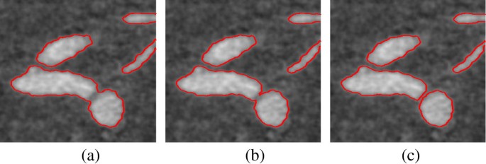
Evolution process of the C-V method ( v = 0.015 × 2552). (a) Initial contour (red curves) with c1(ϕ0) = 158.59 and c2 (ϕ0) = 73.32. (b) Intermediate segmentation result at 240th iterations (c1 (ϕ240) = 161.11, c2 (ϕ240) = 73.74). (c) Final segmentation result at 480th iterations (c1(ϕ480) = 162.54, c2(ϕ480) = 73.95).
-
Thirdly, Equation (15) itself depends on ϕn(x, y) due to c1(ϕn) and c2 (ϕn); thus, the solutions of Equation (15) with the initial condition ϕ(0, x, y) = ϕn(x, y) are more dependent on ϕn(x, y). This implies that the C-V method may be sensitive to contour initialization to some extent. In order to test the sensitivity of the C-V method to contour initialization, we demonstrate the case of three real images with five different initial contours, as shown in Figures 3, 4, 5. For the detailed description, we will give more in Section 4.
Figure 3 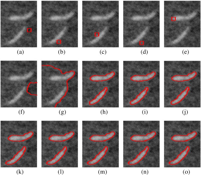
Segmentation results of both methods for a vascular biopsy image. The first row (a to e): original images and initial contours. The second row (f to j): final results of the C-V method (left to right: 4,000, 2,000, 2,300, 600, and 95 iterations). The third row (k to o): final results of our method (14 iterations).
Figure 4 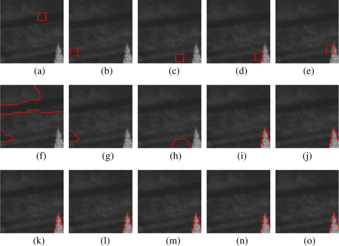
Applications of both methods for an aerial image. The first row (a to e): original images and initial contours. The second row (f to j): final segmentation results of the C-V method (left to right: 3,300, 1,500, 1,500, 260, 70 iterations); the third row (k to o): final segmentation results of our method (one iteration).
Figure 5 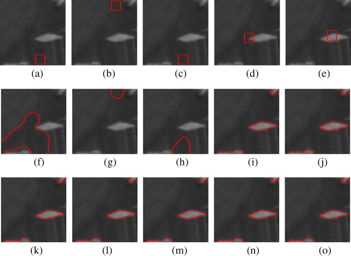
Segmentation results of both methods for a real image with low contrast and multiple objects. The first row (a to e): original images and initial contours. The second row (f to j): final results of the C-V method (left to right: 7,900, 5,000, 2,500, 320, and 80 iterations). The third row (k to o): final results of our method (three iterations).


3.2 The proposed method
We present a new method that implements the piecewise constant M-S functional (2) for two-phase image segmentation, which completely avoids the need of alternating optimization procedure.
The two-phase piecewise constant M-S model (2) is a variational problem for approximating a given two-phase image by a piecewise constant image building up two class of constant regions. This actually tries to find the best ‘cartoon-like’ (i.e. piecewise constant) approximation of minimal complexity for a given image. Once such an approximation is constructed, the homogeneous regions and their boundaries become obvious. Based on the above facts, we present a two-step algorithm for the two-phase piecewise constant M-S model.
Firstly, we consider a two-phase image to be segmented as a data set X. According to the definition of two-phase, the data set X can be separated into two groups by the HCM algorithm; let m1 and m2 be the averages of the two groups, respectively. The values m1 and m2 equal approximately to the intensity means of foreground and background in the image, respectively.
Secondly, similar to the piecewise constant M-S functional (2), we define the following energy functional:
where Ω1 and Ω2 is the interior and the exterior regions of C, respectively. Note that the energy F(C) is only the functional with respect to C.
To handle topological changes, the energy F(C) is then incorporated into a variational level set formulation with an extra internal energy. In other word, the contour C is represented by a level set function, and the minimization of the energy over level set functions is performed by solving a level set evolution equation.
According to the level set method [10, 11], the curve C is represented implicitly by the zero level set of a level set function ϕ : Ω → ℝ that is positive in the interior and negative in the exterior of the contour C. Let H(z) be the Heaviside function, and then the functional (16) can be expressed as
where M1(ϕ) = H(ϕ), M2(ϕ) = 1−H(ϕ). Because the functional (17) only contains an unknown variable ϕ, we can simply minimize F(ϕ) with respect to ϕ.
To preserve the regularity of the level set function, we add an extra internal energy [31]:
to the energy F(ϕ) in (17). The level set regularization term P(ϕ) penalizes the deviation of the level set function ϕ from a signed distance function to avoid the re-initialization procedure [31].
Therefore, the overall energy functional in level set framework is given by
where λ > 0 is a parameter. For practical and feasible implementation, the Heaviside function H(z) has to be approximated by a smooth function H ε (z) given typically by
So, the overall energy functional (19) can then be rewritten as
Minimizing the energy functional (21) by the gradient decent method, we obtain the partial differential equation for ϕ as follows:
with the initial condition ϕ(0, x, y) = ϕ(x, y) and the zero Neumann boundary condition, where is a smooth Dirac function.
4 Implementation and experimental results
The level set evolution in Equation (22) is implemented using a simple finite differencing (forward-time central-space finite difference scheme). All the spatial partial derivatives ∂ϕ/∂x and ∂ϕ/∂y are approximated by the central difference, and the temporal partial derivative ∂ϕ/∂t is discretized as the forward difference. The approximation of Equation (22) can be simply written as
where with k ≥ 0 and is the approximation of the right-hand side in Equation (22) by the above spatial difference scheme. For pixels on the borders of the test images, we take a mirror reflection in all experiments.
To make a fair comparison for the C-V method, we added the internal energy (18) into the functional (5) to avoid the re-initialization step. In our implementation, for the C-V method and proposed method, the initial level set function ϕ0(x, y) is simply chosen as a binary step function as in [31], which takes a positive constant value ρ inside a region ω ⊂ Ω and a negative constant value − ρ outside ω. We choose ρ = 2 for the experiments in this paper.
Unless otherwise specified, we use the following default parameter values for our method: ∆t = 0.1 (time step), ∆x = ∆y = 1 (space step), ε = 1 for the smooth Dirac function, λ = 0.04 for the level set regularization parameter. Besides, for the sake of simplicity, we set v = 0.002 × 2552 for the length parameter. Generally, if v is too small, the robustness to noise may be reduced; if v is too large, the excessive segmentation boundaries may be generated in final segmentation results. Here, we fix v = 0.002 × 2552 since the good segmentation results are obtained for most of the experiments in this paper. In applications, the v value should be selected according to the noise level.
For all experiments, the initial contours are chosen as squares with side length of five pixels, located at the centre of image domain (excluding Figures 2, 3, 4, 5). For the C-V method, the parameters are referred to [12]. We record the iteration number and the CPU time from our experiments with Matlab codes run on an PC, with AMD Athlon (tm) 2.70 GHz CPU, 2.00 GB memory, and Matlab 7.4 on Windows 7.
We will use the dice similarity coefficient (DSC) metric [32] to evaluate quantitatively the performances of both methods. S1 and S2 represent a given baseline foreground region (e.g. true object) and the foreground region found by the model, respectively, then the DSC metric is defined as
where N(⋅) indicates the number of pixels in the enclosed region. The closer the DSC value to 1, the better the segmentation; a perfect segmentation will give DSC = 1.
First, we evaluate quantitatively the proposed method according the DSC metric. We test on four synthetic images with additive Gaussian noise, which are shown in Figure 6; the four synthetic images are originally noise-free, which contain only two distinct gray levels. The true objects can be immediately obtained from the original images by a thresholding algorithm. As shown in the second row of Figure 6, the proposed method obtains satisfactory results visually. By quantitative comparison we can show that the proposed method really produces the perfect results for four images with noise (see Table 1).

Segmentation results of our method for four synthetic images added additive Gaussian noise. Top row (a to d): original images and initial contours. Bottom row (e to h): final results.
Second, we show the segmentation results of both the proposed and C-V methods for some synthetic images (see Figure 7) and real images (see Figures 3, 4, 5).

Segmentation results of both methods for five synthetic images. Top row (a to e): original images and initial contours. Middle row (f to j): final results of the C-V method (left to right: 15, 30, 24, 7, and 14 iterations). Bottom row (k to o): final results of our method (one iteration).
In Figure 7, the proposed method is applied to segment five synthetic images and compares with the C-V method visually and quantitatively. It is clearly seen from Figure 7 that the proposed method obtains the satisfactory segmentation results for five synthetic images, which are almost the same as the C-V method visually. The quantitative comparison of both methods is given in Table 2, in which the results of the C-V method are regarded as baseline foreground regions (we take ten iterations (for the inner loop) to obtain the optimal results of the C-V method; but we still take one iteration (just as done in [12]) to achieve the optimal speed of the C-V method). By quantitative comparison, the proposed method achieves the same results as the C-V method for the three images and almost the same results for the other two images. Moreover, Table 2 demonstrates that the proposed method provides the faster converging speed than the C-V method.
In Figures 3, 4, 5, we test the sensitivity of both methods to the locations of initial contours, where the initial contour is chosen as a square. Test images are a vascular biopsy image (94 × 123), an aerial image (250 × 250) and a real image with low contrast and multiple objects (184 × 184). Figure 3 shows the segmentation results of a vascular biopsy image for five different initializations (same size but different location). The original image along with five distinct initial contours is listed in the first row of Figure 3. From Figure 3f,g,h,i,j, we observe that the C-V method fails to segment the vascular biopsy image for the first two initial contours; by contrast, the proposed method segment correctly the vascular biopsy image after the same iterations for the five initial contours. Besides, although the C-V method captures all objects for other three locations (see Figure 3h,i,j), the iteration numbers vary greatly from 95 to 2,300 for the vascular biopsy image.
Figure 4 shows the results of both methods for an aerial image. The initial contours have different location, as shown in Figure 4a,b,c,d,e. It can be seen from Figure 4f,g,h,i,j that the C-V method cannot segment correctly the aerial image for first three initial contours although it produces satisfactory results for the last two contours (which also need different iterations). As shown in Figure 4k,l,m,n,o, the proposed method has obtained the satisfactory segmentation result after single iteration for each of the five initial locations.
In Figure 5, we demonstrate the segmentation results of both methods for an image with low contrast and multiple objects. The initial contours over the original image are shown in Figure 5a,b,c,d,e. From Figure 5f,g,h,i,j, we observe that the C-V method fails to segment the real image for the first three initial contours while it captures better the object for the last two initial contours (Figure 5i,j). The proposed method has successfully extracted all objects of interest after the same iterations for the five initial contours (see Figure 5k,l,m,n,o). Experiments in Figures 3, 4, 5 show that the proposed method really allows for more flexible initialization than the original C-V method.
Third, the next two experiments show the segmentation results of the proposed and Bresson et al.'s methods [20] for some real images (see Figures 8 and 9). To make a fair comparison, we experimentally choose the best parameters for the Bresson et al.'s method.

Applications of the proposed and Bresson et al.'s methods to four infrared images. The first row (a to d): original images. The second row (e to h): final segmentation results of the Bresson et al.'s method. The third row (i to l): final segmentation results of the proposed method.

Segmentation results of the proposed and Bresson et al.'s methods for four real images. Top row (a to d): original images. Middle row (e to h): final results of the Bresson et al.'s method. Bottom row (i to l): final results of the proposed method.
Figure 8 shows the detective results of the proposed and Bresson et al.'s methods for four infrared images. Because of the limitation in thermal imaging and the actual surroundings' conflicts, infrared images always suffer from low contrast and complex (noisy) background. In the proposed method, we use v = 0.015 × 2552 for the second and third images. Figure 8a,b,c,d is the original image. As shown in Figure 8i,j,k,l, the proposed method successfully detects the objects for all these images. By comparison, the proposed method achieves almost the same results as the Bresson et al.'s method (see Figure 8e,f,g,h); however, we observe from Table 3 that the iteration numbers and CPU times of the proposed model are less than the Bresson et al.'s method.
In Figure 9, we apply the proposed and Bresson et al.'s methods to the four real images with complex background or multiple objects. The four images, which are plotted in Figure 9a,b,c,d, are two real images with complex background, a DNA channel image with blurry edges and multiple objects, and an aerial image with low contrast and multiple objects. It can be seen from the second and third rows of Figure 9 that both methods successfully extract the object boundaries with similar results. Besides, the proposed method provides the faster converging speed compared to the Bresson et al.'s method, as shown in Table 4.
The last experiment shows the segmentation results using C-V method, Bresson et al.'s method and the proposed method for four medical images (see Figure 10) and three real-world pictures (see Figure 11). Figure 10a,b,c,d shows a breast cyst image with imaging artifacts, a skin lesion image contaminated by texture tissue, a MR heart image with clutter noise and a cell image with multiple objects. It is seen from Figure 10m,n,o,p that the proposed method obtains the satisfactory segmentation results for four medical images, which are similar to the C-V method (Figure 10e,f,g,h) and Bresson et al.'s method (Figure 10i,j,k,l). The iterations and CPU times by the three methods are given in Table 5, which shows that the Bresson et al.'s method has less iterations and CPU times than the C-V method; furthermore, the proposed method, only through a few iterations, can achieve satisfactory segmentation results for these images.

Segmentation results of proposed, C-V and Bresson et al.'s methods on four real medical images. First row (a to d): original images. Second row (e to h): final results of the C-V method. Third row (i to l): final results of the Bresson et al.'s method. Fourth row (m to p): final results of the proposed method.

Segmentation results of proposed, C-V and Bresson et al.'s methods on three real-world pictures. First column (a,e,i): original pictures. Second column (b,f,j): final results of the C-V method. Third column (c,j,k): final results of the Bresson et al.'s method. Fourth column (d,h,l): final results of the proposed method.
Here, we also provided more experiments on the three different types of real-world pictures to further demonstrate the performance of three methods, as shown in Figure 11. The three pictures, which are plotted in Figure 11a,e,i, are a real lotus picture, a real garden picture and a cameraman picture. In the proposed method, we use v = 0.08 × 2552 for the first two pictures and v = 0.03 × 2552 for the third picture. The lotus picture has complex background and object shapes. The garden picture has complex background; the segmentation process may be influenced by the existences of wall, gate and grass. The cameraman picture is a well-known picture and has been used in the Bresson et al.'s method. From the fourth column of Figure 11, we can see that the proposed method obtains the satisfactory segmentation results for three real-world pictures. The results using our method are similar to those of the C-V and Bresson et al.'s methods (see the second and third columns of Figure 11); however, the proposed method has less iterations and CPU times than the other two methods for the three pictures (see Table 6). It is clear that the proposed method is more efficient than the C-V method and Bresson et al.'s method.
5 Conclusions
In this paper, we present a very efficient method to solve the two-phase piecewise constant M-S model for image segmentation within the level set framework. Unlike the well-known C-V method using alternating optimization, we first use a clustering algorithm to obtain a ‘cartoon-like’ approximation of minimal complexity to a given image. From the cartoon-like image, we can approximately obtain the intensity means of foreground and background in the image. The M-S functional is reduced to the function of single variable (level set function) and so does not need to use alternating optimization. Numerical results demonstrated some advantages of the proposed method over the C-V method, such as robustness to the locations of initial contour and the high computation efficiency.
References
Carriero M, Leaci A, Tomarelli F: Calculus of variations and image segmentation. J Physiol Paris 2003, 97: 343-353. 10.1016/j.jphysparis.2003.09.008
Chan TF, Moelich M, Sandberg B: Some Recent Developments in Variational Image Segmentation, Part III. Heidelberg: Springer; 2007:175-210.
Mumford D, Shah J: Optimal approximation by piecewise smooth functionals and associated variational problems. Commun. Pure Appl. Math. 1989, 42(5):577-685. 10.1002/cpa.3160420503
Chambolle A: Image segmentation by variational methods: Mumford and Shah functional and the discrete approximations. SIAM J. Appl. Math. 1995, 55(3):827-863. 10.1137/S0036139993257132
Tsai A, Yezzi A, Willsky AS: Curve evolution implementation of the Mumford-Shah functional for image segmentation, denoising, interpolation, and magnification. IEEE Trans Image Process 2001, 10(8):1169-1186. 10.1109/83.935033
Gao S, Bui TD: Image segmentation and selective smoothing by using Mumford-Shah model. IEEE Trans Image Process 2005, 14(10):1537-1549.
Brox T, Cremers D: On local region models and a statistical interpretation of the piecewise smooth Mumford-Shah functional. Int. J. Comput. Vis. 2009, 84: 184-193. 10.1007/s11263-008-0153-5
Geman S, Geman D: Stochastic relaxation, Gibbs distributions, and the Bayesian restoration of images. IEEE Trans. Pattern Anal. Machine Intell. 1984, 6(6):721-741.
Blake A, Zisserman A: Visual reconstruction. 1987. . Accessed 1987 http://www.research.microsoft.com/en-us/um/people/ablake/papers/VisualReconstruction
Osher S, Sethian JA: Fronts propagating with curvature-dependent speed: algorithms based on Hamilton-Jacobi formulations. J Comput Phys 1988, 79: 12-49. 10.1016/0021-9991(88)90002-2
Sethian JA: Level Set Methods and Fast Marching Methods. Cambridge: Cambridge University Press; 1999.
Chan TF, Vese LA: Active contours without edges. IEEE Trans Image Process 2001, 10(2):266-277. 10.1109/83.902291
Chan TF, Vese LA: A multiphase level set framework for image segmentation using the Mumford and Shah model. Int. J. Comput. Vis. 2002, 50(3):271-293. 10.1023/A:1020874308076
Lie J, Lysaker M, Tai XC: A binary level set model and some applications to Mumford-Shah image segmentation. IEEE Trans Image Process 2006, 15(5):1171-1181.
Cremers D, Rousson M, Deriche R: A review of statistical approaches to level set segmentation: integrating color, texture, motion and shape. Int. J. Comput. Vis. 2007, 72(2):195-215. 10.1007/s11263-006-8711-1
Wang Y, He C: Image segmentation algorithm by piecewise smooth approximation. EURASIP J. Image Vid. 2012, 2012: 16. 10.1186/1687-5281-2012-16
He C, Wang Y, Chen Q: Active contours driven by weighted region-scalable fitting energy based on local entropy. Signal Process. 2012, 92: 587-600. 10.1016/j.sigpro.2011.09.004
Shen JH: Γ-Convergence Approximation to Piecewise Constant Mumford-Shah Segmentation. Heidelberg: Springer; 2005:499-506.
Esedoĝlu S, Tsai YHR: Threshold dynamics for the piecewise constant Mumford-Shah functional. J Comput Phys 2006, 211: 367-384. 10.1016/j.jcp.2005.05.027
Bresson X, Esedoĝlu S, Vandergheynst P, Thiran JP, Osher S: Fast global minimization of the active contour/snake model. J. Math. Imaging Vis 2007, 28: 151-167. 10.1007/s10851-007-0002-0
Bezdek JC, Hathaway RJ, Howard RE, Wilson CA, Windham MP: Local convergence analysis of a grouped variable version of coordinate descent. J. Optimiz. Theory App. 1987, 54(3):471-477. 10.1007/BF00940196
Bezdek JC, Hathaway RJ: Some Notes on Alternating Optimization. Heidelberg: Springer; 2002:288-300.
Ambrosio L, Tortorelli VM: Approximation of functionals depending on jumps by elliptic functionals via Γ-convergence. Comm. Pure Appl. Math. 1990, 43: 999-1036. 10.1002/cpa.3160430805
Aubert G, Feraud BL, March R: An approximation of the Mumford-Shah energy by a family of discrete edge-preserving functional. Nonlinear Anal. -Thero. 2006, 64(9):1908-1930. 10.1016/j.na.2005.07.028
Yu L, Wang Q, Wu L, Xie J: A Mumford-Shah model on lattice. Image Vision Comput. 2008, 26: 1663-1669. 10.1016/j.imavis.2008.04.024
Dubes R, Jain AK: Clustering methodology in exploratory data analysis. Adv. Comput. 1980, 19: 113-228.
Jain AK, Murty MN, Flynn PJ: Data clustering: a review. ACM Comput. Surv. 1999, 31(3):264-323. 10.1145/331499.331504
Macqueen J: Some methods for classification and analysis of multivariate observations. In Fifth Berkeley Symposium on Mathematical Statistics and Probability. Berkeley: the University of California; 1967.
Bezdek JC: A convergence theorem for the fuzzy ISODATA clustering algorithms. IEEE Trans. Pattern Anal. Machine Intell. 1980, PAMI-2(1):1-8.
Krishnapuram R, Keller JM: A possibilistic approach to clustering. IEEE Trans. Fuzzy Systems 1993, 1(2):98-110. 10.1109/91.227387
Li C, Xu C, Fox MD: Level set evolution without re-initialization: a new variational formulation, in Proceedings of IEEE Conference on Computer Vision and Pattern Recognition (CVPR), 1st edn. San Diego; 2005:430-436.
Shattuck DW, Sandor-Leahy SR, Schaper KA, Rottenberg DA, Leahy RM: Magnetic resonance image tissue classification using a partial volume model. Neuroimage 2001, 13: 856-876.
Acknowledgements
The authors would like to thank the anonymous reviewers for their valuable comments and suggestions to improve this paper. This work was supported by Chongqing Education Committee Science Research Project No. KJ130604.
Author information
Authors and Affiliations
Corresponding author
Additional information
Competing interests
The authors declare that they have no competing interests.
Authors’ original submitted files for images
Below are the links to the authors’ original submitted files for images.
Rights and permissions
Open Access This article is distributed under the terms of the Creative Commons Attribution 2.0 International License (https://creativecommons.org/licenses/by/2.0), which permits unrestricted use, distribution, and reproduction in any medium, provided the original work is properly cited.
About this article
Cite this article
Chen, Q., He, C. Integrating clustering with level set method for piecewise constant Mumford-Shah model. J Image Video Proc 2014, 1 (2014). https://doi.org/10.1186/1687-5281-2014-1
Received:
Accepted:
Published:
DOI: https://doi.org/10.1186/1687-5281-2014-1